This code demonstrates individual tree segmentation (ITS) using LiDAR data. It covers CHM-based and point cloud-based methods for tree detection and segmentation. The code also shows how to extract metrics at the tree level and visualize them.
Environment
# Clear environmentrm(list =ls(globalenv()))# *Ensure 'concaveman' is installed for tree segmentation*if (!requireNamespace("concaveman", quietly =TRUE)) {install.packages("concaveman")}# Load all required packageslibrary(concaveman)library(lidR)library(sf)library(terra)# Read in LiDAR file and set some color paletteslas <-readLAS("data/zrh_norm.laz")
col <-height.colors(50)col1 <-pastel.colors(900)
CHM based methods
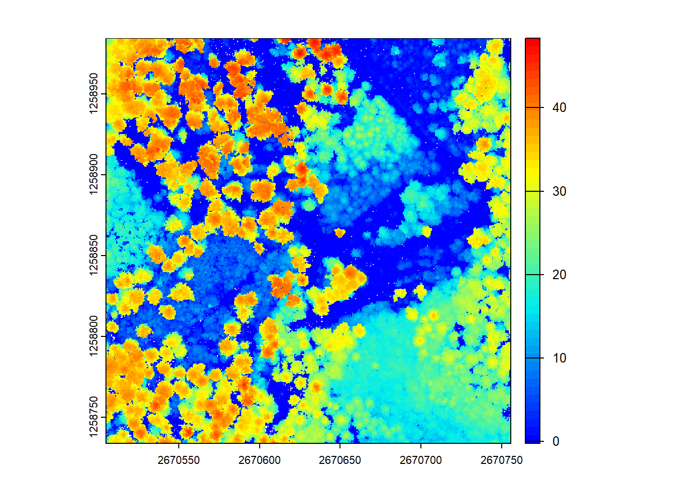
We start by creating a Canopy Height Model (CHM) from the LiDAR data. The rasterize_canopy() function generates the CHM using a specified resolution (res) and a chosen algorithm, here p2r(0.15), to compute the percentiles.
# Generate CHMchm <-rasterize_canopy(las = las, res =0.5, algorithm =p2r(0.15))plot(chm, col = col)
After building the CHM, we visualize it using a color palette (col).
Optionally smooth the CHM
Optionally, we can smooth the CHM using a kernel to remove small-scale variations and enhance larger features like tree canopies.
# Generate kernel and smooth chmkernel <-matrix(1, 3, 3)schm <- terra::focal(x = chm, w = kernel, fun = median, na.rm =TRUE)plot(schm, col = col)
Here, we smooth the CHM using a median filter with a 3x3 kernel. The smoothed CHM (schm) is visualized using a color palette to represent height values.
Tree detection
Next, we detect tree tops using the smoothed CHM. The locate_trees() function identifies tree tops based on local maxima.
# Detect treesttops <-locate_trees(las = schm, algorithm =lmf(ws =2.5))ttops#> Simple feature collection with 2694 features and 2 fields#> Attribute-geometry relationships: constant (2)#> Geometry type: POINT#> Dimension: XYZ#> Bounding box: xmin: 2670505 ymin: 1258734 xmax: 2670755 ymax: 1258984#> Projected CRS: CH1903+ / LV95#> First 10 features:#> treeID Z geometry#> 1 1 37.080 POINT Z (2670514 1258984 37...#> 2 2 38.230 POINT Z (2670534 1258984 38...#> 3 3 41.185 POINT Z (2670555 1258984 41...#> 4 4 3.915 POINT Z (2670578 1258984 3....#> 5 5 6.090 POINT Z (2670591 1258984 6.09)#> 6 6 37.885 POINT Z (2670597 1258984 37...#> 7 7 46.160 POINT Z (2670614 1258984 46...#> 8 8 46.645 POINT Z (2670617 1258984 46...#> 9 9 9.170 POINT Z (2670652 1258984 9.17)#> 10 10 3.075 POINT Z (2670687 1258984 3....plot(chm, col = col)plot(ttops, col ="black", add =TRUE, cex =0.5)
The detected tree tops (ttops) are plotted on top of the CHM (chm) to visualize their positions.
Segmentation
Now, we perform tree segmentation using the detected tree tops. The segment_trees() function segments the trees in the LiDAR point cloud based on the previously detected tree tops.
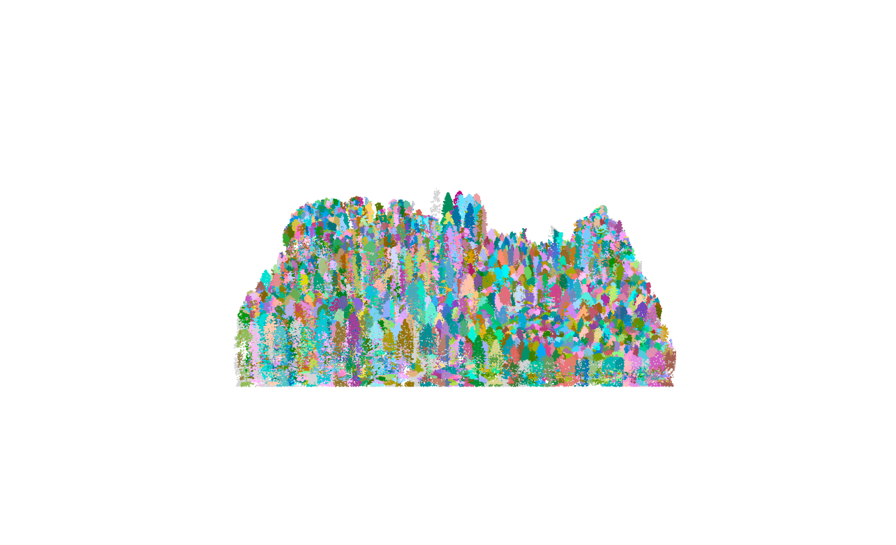
# Segment trees using dalpontelas <-segment_trees(las = las, algorithm =dalponte2016(chm = schm, treetops = ttops))
# Count number of trees detected and segmentedlength(unique(las$treeID) |>na.omit())#> [1] 2653
# Visualize all treesplot(las, color ="treeID")
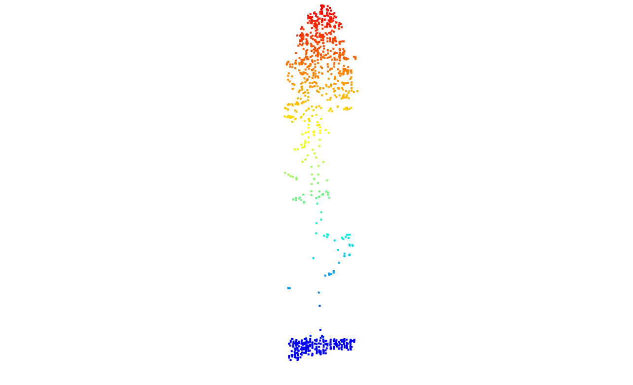
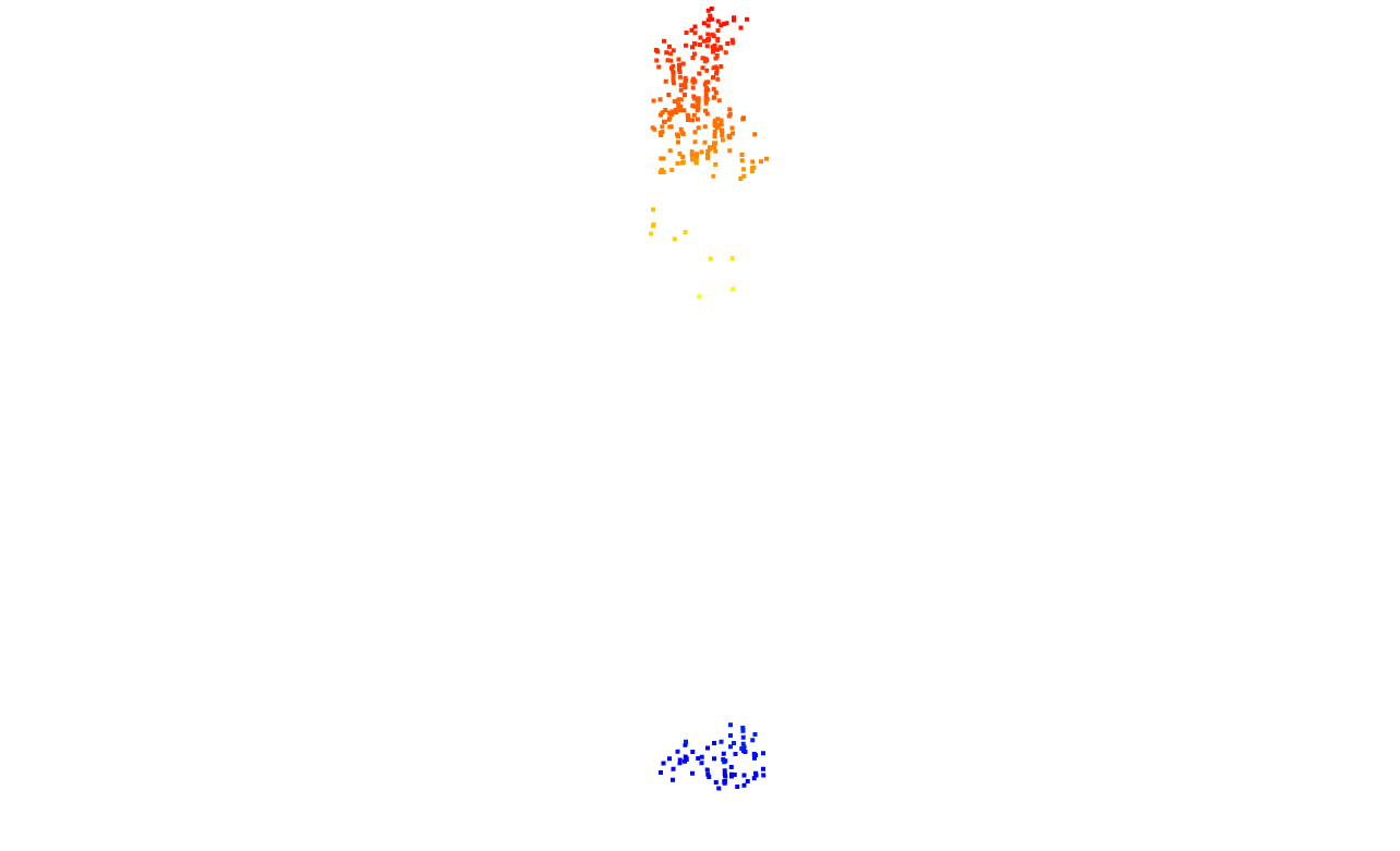
# Select trees by IDtree25 <-filter_poi(las = las, treeID ==25)tree125 <-filter_poi(las = las, treeID ==125)
plot(tree25, size =4)
plot(tree125, size = 3)
After segmentation, we count the number of trees detected and visualize all the trees in the point cloud. We then select two trees (tree25 and tree125) and visualize them individually.
Variability and testing
Forests are highly variable! This means that some algorithms and parameters will work better than others depending on the data you have. Play around with algorithms and see which works best for your data.
Working with rasters
The lidR package is designed for point clouds, but some functions can be applied to raster data as well. Here, we show how to extract trees from the CHM without using the point cloud directly.
# Generate rasterized delineationtrees <-dalponte2016(chm = chm, treetops = ttops)() # Notice the parenthesis at the endtrees#> class : SpatRaster #> dimensions : 501, 501, 1 (nrow, ncol, nlyr)#> resolution : 0.5, 0.5 (x, y)#> extent : 2670505, 2670756, 1258734, 1258985 (xmin, xmax, ymin, ymax)#> coord. ref. : CH1903+ / LV95 (EPSG:2056) #> source(s) : memory#> name : Z #> min value : 1 #> max value : 2694plot(trees, col = col1)plot(ttops, add =TRUE, cex =0.5)#> Warning in plot.sf(ttops, add = TRUE, cex = 0.5): ignoring all but the first#> attribute
We create tree objects (trees) using the dalponte2016 algorithm with the CHM and tree tops. The resulting objects are visualized alongside the detected tree tops.
Point-cloud based methods (no CHM)
In this section, we will explore tree detection and segmentation methods that do not require a CHM.
Tree detection
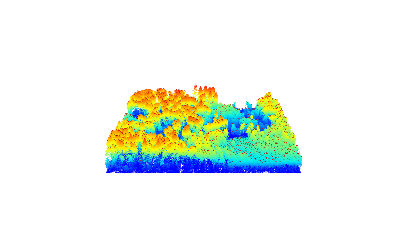
We begin with tree detection using the local maxima filtering (lmf) algorithm. This approach directly works with the LiDAR point cloud to detect tree tops.
We detect tree tops using the lmf algorithm and visualize them in 3D by adding the tree tops to the LiDAR plot.
Tree segmentation
Next, we perform tree segmentation using the li2012 algorithm, which directly processes the LiDAR point cloud.
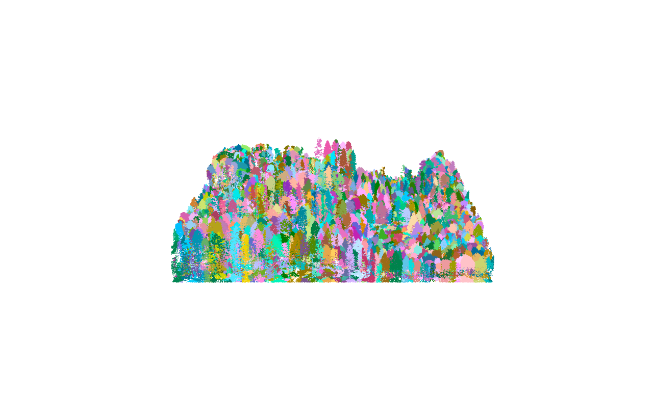
# Segment using lilas <-segment_trees(las = las, algorithm =li2012())
plot(las, color ="treeID")# This algorithm does not seem pertinent for this dataset.
The li2012 algorithm segments the trees in the LiDAR point cloud based on local neighborhood information. However, it may not be optimal for this specific dataset.
Extraction of metrics
We will extract various metrics from the tree segmentation results.
Using crown_metrics()
The crown_metrics() function extracts metrics from the segmented trees using a user-defined function. We use the length of the Z coordinate to obtain the tree height as an example.
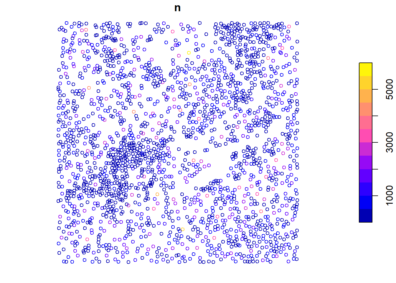
# Generate metrics for each delineated crownmetrics <-crown_metrics(las = las, func =~list(n =length(Z)))metrics#> Simple feature collection with 2018 features and 2 fields#> Geometry type: POINT#> Dimension: XYZ#> Bounding box: xmin: 2670505 ymin: 1258734 xmax: 2670755 ymax: 1258984#> z_range: zmin: 2.02 zmax: 48.31#> Projected CRS: CH1903+ / LV95#> First 10 features:#> treeID n geometry#> 1 1 1140 POINT Z (2670616 1258984 48...#> 2 2 3404 POINT Z (2670625 1258975 47...#> 3 3 1748 POINT Z (2670634 1258983 46...#> 4 4 1579 POINT Z (2670642 1258975 46...#> 5 5 2533 POINT Z (2670626 1258904 46...#> 6 6 1573 POINT Z (2670647 1258978 45...#> 7 7 1922 POINT Z (2670591 1258771 45.3)#> 8 8 5630 POINT Z (2670642 1258953 45...#> 9 9 1578 POINT Z (2670556 1258741 44...#> 10 10 1283 POINT Z (2670652 1258949 44...plot(metrics["n"], cex =0.8)
We calculate the number of points (n) in each tree crown using a user-defined function, and then visualize the results.
Applying user-defined functions
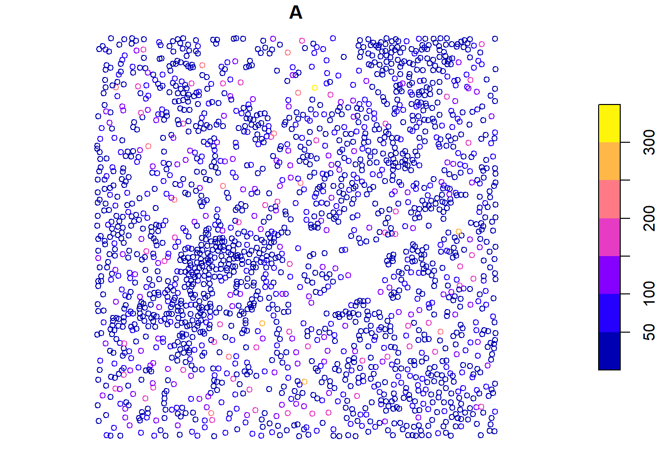
We can map any user-defined function at the tree level using the crown_metrics() function, just like pixel_metrics(). Here, we calculate the convex hull area of each tree using a custom function f() and then visualize the results.
# User defined function for area calculationf <-function(x, y) {# Get xy for tree coords <-cbind(x, y)# Convex hull ch <-chull(coords)# Close coordinates ch <-c(ch, ch[1]) ch_coords <- coords[ch, ]# Generate polygon p <- sf::st_polygon(list(ch_coords))#calculate area area <- sf::st_area(p)return(list(A = area))}# Apply user-defined functionmetrics <-crown_metrics(las = las, func =~f(X, Y))metrics#> Simple feature collection with 2018 features and 2 fields#> Geometry type: POINT#> Dimension: XYZ#> Bounding box: xmin: 2670505 ymin: 1258734 xmax: 2670755 ymax: 1258984#> z_range: zmin: 2.02 zmax: 48.31#> Projected CRS: CH1903+ / LV95#> First 10 features:#> treeID A geometry#> 1 1 117.07885 POINT Z (2670616 1258984 48...#> 2 2 225.63075 POINT Z (2670625 1258975 47...#> 3 3 152.64110 POINT Z (2670634 1258983 46...#> 4 4 92.06825 POINT Z (2670642 1258975 46...#> 5 5 112.30745 POINT Z (2670626 1258904 46...#> 6 6 78.93495 POINT Z (2670647 1258978 45...#> 7 7 153.69045 POINT Z (2670591 1258771 45.3)#> 8 8 305.83890 POINT Z (2670642 1258953 45...#> 9 9 104.63505 POINT Z (2670556 1258741 44...#> 10 10 166.12705 POINT Z (2670652 1258949 44...plot(metrics["A"], cex =0.8)
3rd party metric packages
Remember that you can use 3rd party packages like lidRmetrics for crown metrics too!
Using pre-defined metrics
Some metrics are already recorded, and we can directly calculate them at the tree level using crown_metrics().
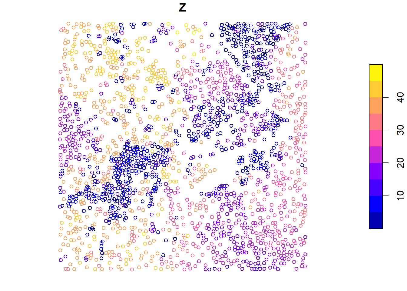
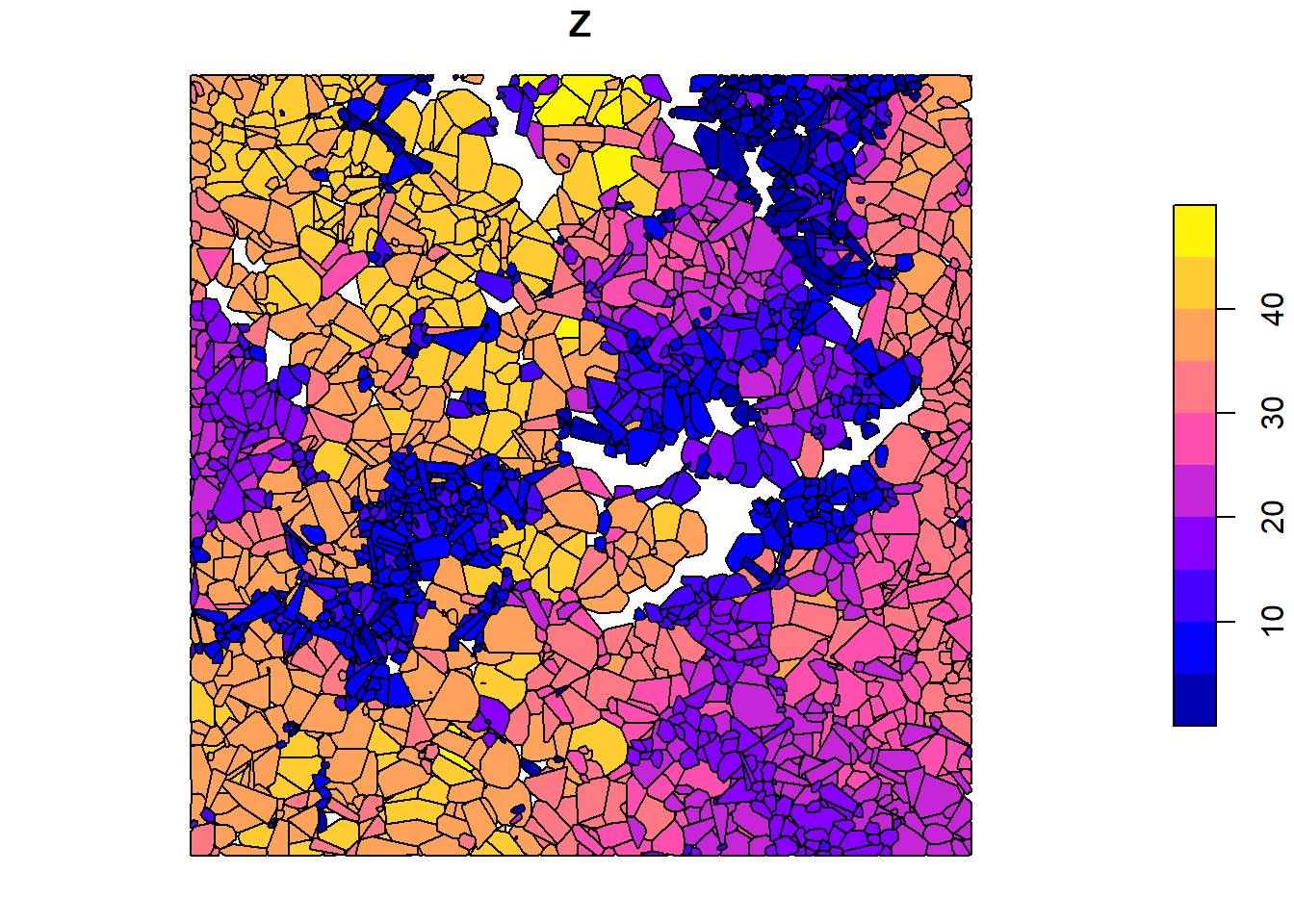
metrics <-crown_metrics(las = las, func = .stdtreemetrics)metrics#> Simple feature collection with 2018 features and 4 fields#> Geometry type: POINT#> Dimension: XYZ#> Bounding box: xmin: 2670505 ymin: 1258734 xmax: 2670755 ymax: 1258984#> z_range: zmin: 2.02 zmax: 48.31#> Projected CRS: CH1903+ / LV95#> First 10 features:#> treeID Z npoints convhull_area geometry#> 1 1 48.31 1140 117.079 POINT Z (2670616 1258984 48...#> 2 2 47.43 3404 225.631 POINT Z (2670625 1258975 47...#> 3 3 46.56 1748 152.641 POINT Z (2670634 1258983 46...#> 4 4 46.46 1579 92.068 POINT Z (2670642 1258975 46...#> 5 5 46.01 2533 112.307 POINT Z (2670626 1258904 46...#> 6 6 45.93 1573 78.935 POINT Z (2670647 1258978 45...#> 7 7 45.30 1922 153.690 POINT Z (2670591 1258771 45.3)#> 8 8 45.27 5630 305.839 POINT Z (2670642 1258953 45...#> 9 9 44.81 1578 104.635 POINT Z (2670556 1258741 44...#> 10 10 44.81 1283 166.127 POINT Z (2670652 1258949 44...# Visualize individual metricsplot(x = metrics["convhull_area"], cex =0.8)
plot(x = metrics["Z"], cex =0.8)
We calculate tree-level metrics using .stdtreemetrics and visualize individual metrics like convex hull area and height.
Delineating crowns
The crown_metrics() function segments trees and extracts metrics at the crown level.
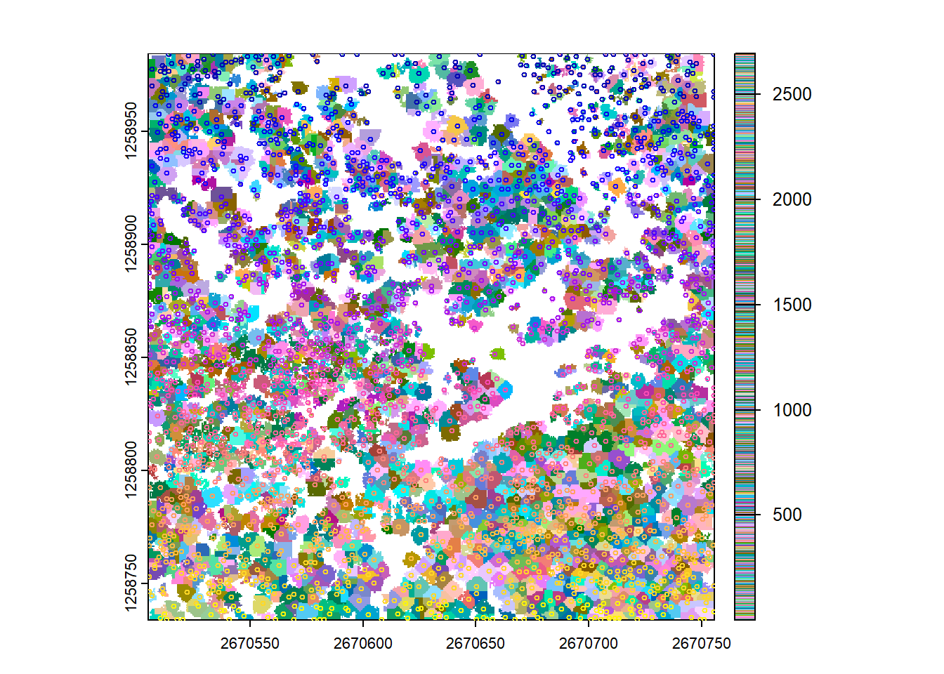
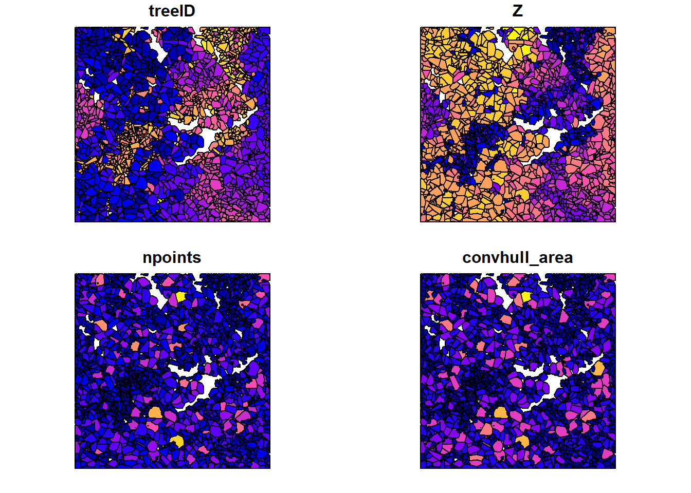
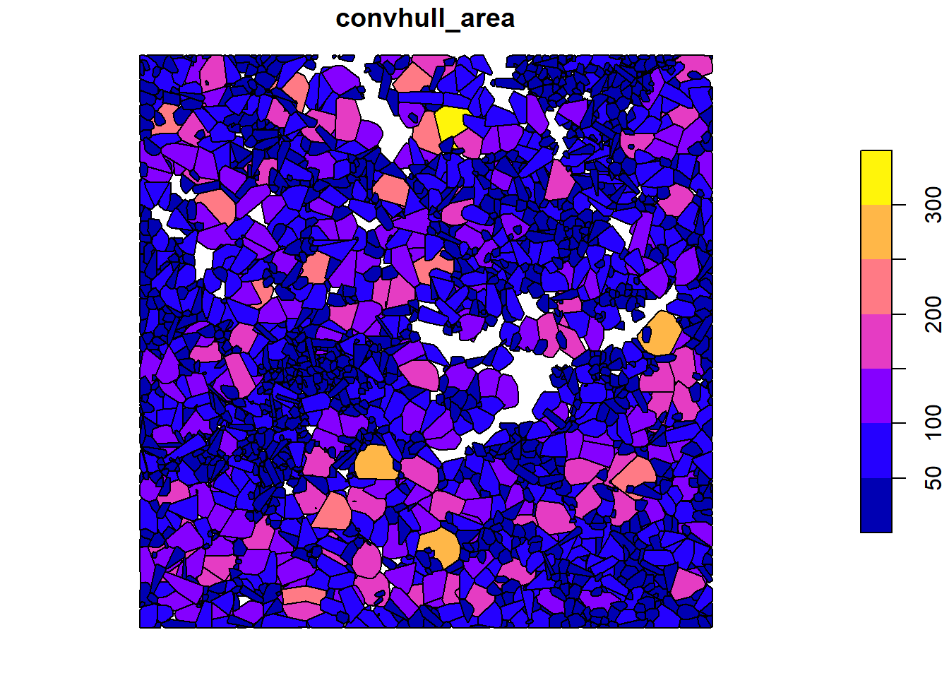
# Visualize individual metrics based on valuesplot(x = cvx_hulls["convhull_area"])
plot(x = cvx_hulls["Z"])
We use crown_metrics() with .stdtreemetrics to segment trees and extract metrics based on crown delineation.
ITD using LAScatalog
In this section, we explore Individual Tree Detection (ITD) using the LAScatalog. We first configure catalog options for ITD.
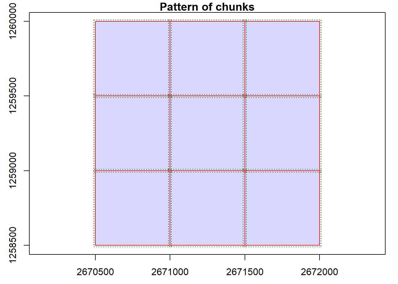
# Load catalogctg <-catalog('data/ctg_norm')# Set catalog optionsopt_filter(ctg) <-"-drop_z_below 0 -drop_z_above 50"opt_select(ctg) <-"xyz"opt_chunk_size(ctg) <-500opt_chunk_buffer(ctg) <-10opt_progress(ctg) <-TRUE# Explicitly tell R to use the is.empty function from the lidR package - avoid terra erroris.empty <- lidR::is.empty# Detect treetops and plotttops <-locate_trees(las = ctg, algorithm =lmf(ws =3, hmin =10))
#> Chunk 1 of 9 (11.1%): state ✓
#>
Chunk 2 of 9 (22.2%): state ✓
#>
Chunk 3 of 9 (33.3%): state ✓
#>
Chunk 4 of 9 (44.4%): state ✓
#>
Chunk 5 of 9 (55.6%): state ✓
#>
Chunk 6 of 9 (66.7%): state ✓
#>
Chunk 7 of 9 (77.8%): state ✓
#>
Chunk 8 of 9 (88.9%): state ✓
#>
Chunk 9 of 9 (100%): state ✓
#>
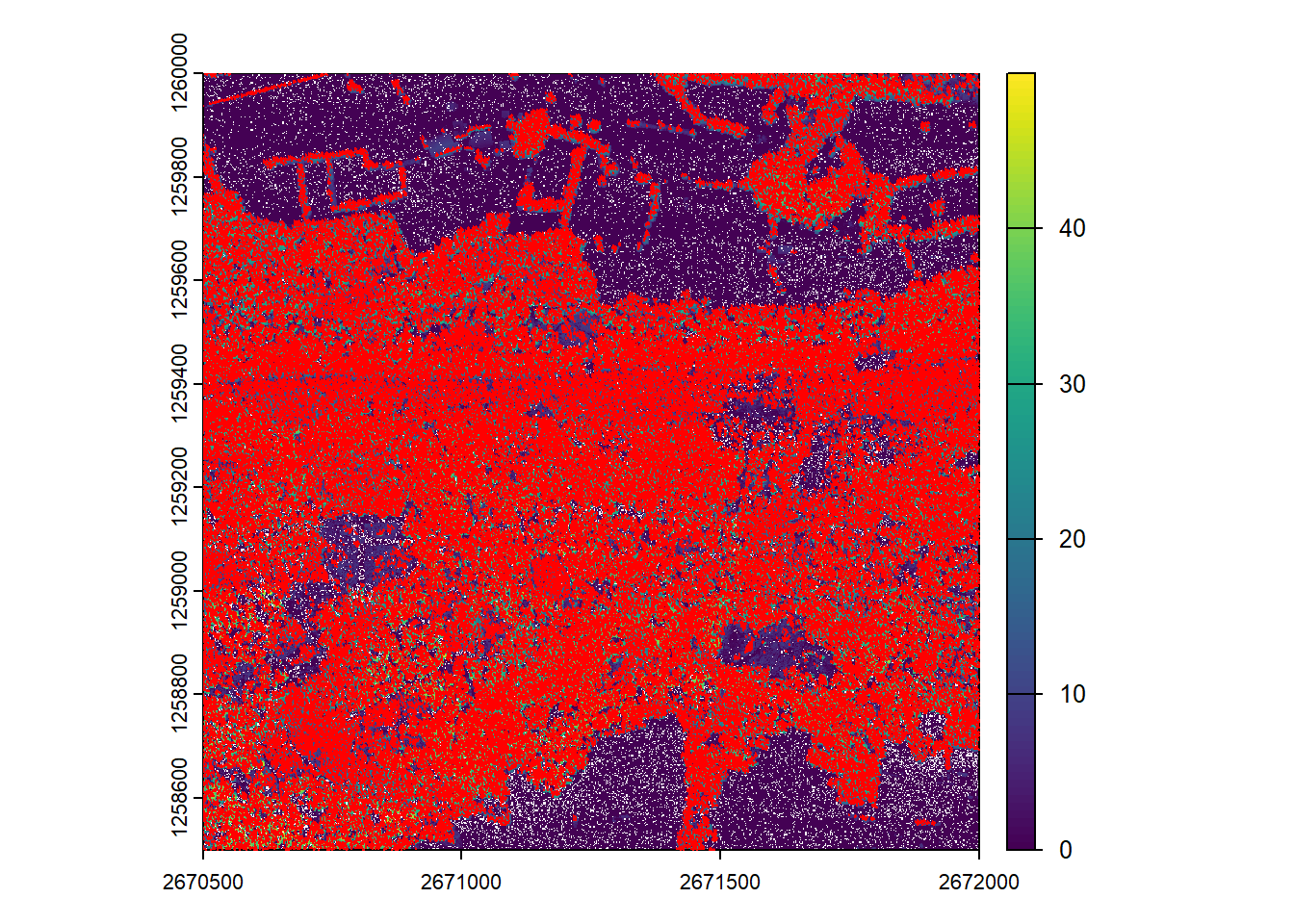
chm <- rasterize_canopy(ctg, algorithm = p2r(), res = 1)
#> Chunk 1 of 9 (11.1%): state ✓
#>

Chunk 2 of 9 (22.2%): state ✓
#>

Chunk 3 of 9 (33.3%): state ✓
#>

Chunk 4 of 9 (44.4%): state ✓
#>

Chunk 5 of 9 (55.6%): state ✓
#>

Chunk 6 of 9 (66.7%): state ✓
#>

Chunk 7 of 9 (77.8%): state ✓
#>

Chunk 8 of 9 (88.9%): state ✓
#>

Chunk 9 of 9 (100%): state ✓
#>

plot(chm)
plot(ttops, add = TRUE, cex = 0.1, col = "red")
Conclusion
This concludes the tutorial on various methods for tree detection, segmentation, and extraction of metrics using the lidR package in R.