# Clear environment
rm(list = ls(globalenv()))

# Load packages
library(lidR)
library(sf)LAScatalog
Relevant resources:
Overview
This code performs various operations on lidar data using LAScatalog functionality. We visualize and inspect the data, validate the files, clip the data based on specific coordinates, generate a Canopy Height Model (CHM), specify processing options, and use parallel computing.
Environment
Basic Usage
In this section, we will cover the basic usage of the lidR package, including reading lidar data, visualization, and inspecting metadata.
If you haven’t downloaded the catalog files yet:
Download additional classified lidar files for 05_engine (.zip, 80 MB) Download additional normalized lidar files for 05_engine (.zip, 78 MB)
Unzip ctg_class.zip and ctg_norm.zip to their respective folders in data/ctg_*
Read catalog from directory of files
We begin by creating a LAS catalog (ctg) from a folder containing multiple .las/.laz files using the readLAScatalog() function.
# Read catalog of files
ctg <- readLAScatalog(folder = "data/ctg_norm")
Catalog information
We can receive a summary about the catalog by calling the object’s name.
ctg
#> class       : LAScatalog (v1.1 format 1)
#> extent      : 2670500, 2672000, 1258500, 1260000 (xmin, xmax, ymin, ymax)
#> coord. ref. : CH1903+ / LV95
#> area        : 2.25 km²
#> points      : 11.25 million points
#> type        : airborne
#> density     : 5 points/m²
#> density     : 2 pulses/m²
#> num. files  : 9
Visualize catalog
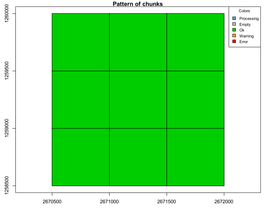
We can visualize the catalog, showing the spatial coverage of the lidar data header extents. Note with chunk = TRUE we see the automatic buffers (dashed line) applied to each tile to avoid edge effects.
plot(ctg, chunk = TRUE)
LAScatalog showing the spatial layout of the individual lidar tiles.
With the mapview package installed, this map can be interactive if we use map = TRUE. Try clicking on a tile to see its header information.
# Interactive
plot(ctg, map = TRUE)LAScatalog using mapview
When all processing is completed without issues, all tiles are colored green.
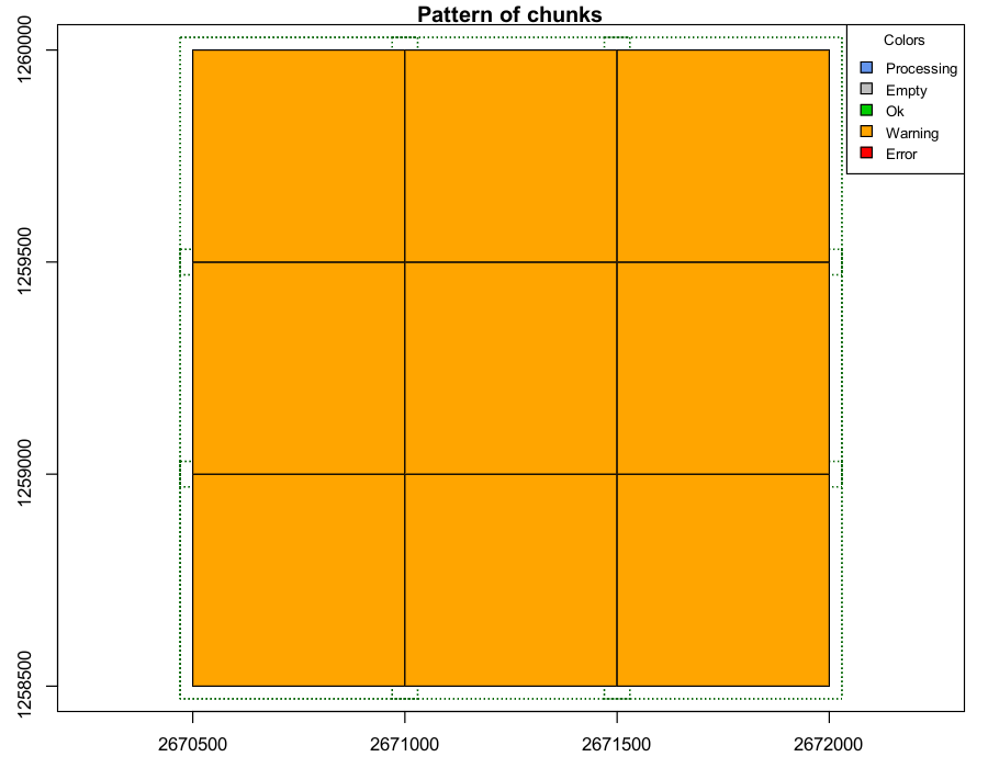
If a process runs but generates a warning for a tile they are coloured yellow. The processing for that tile may have completed, but it requires inspection.
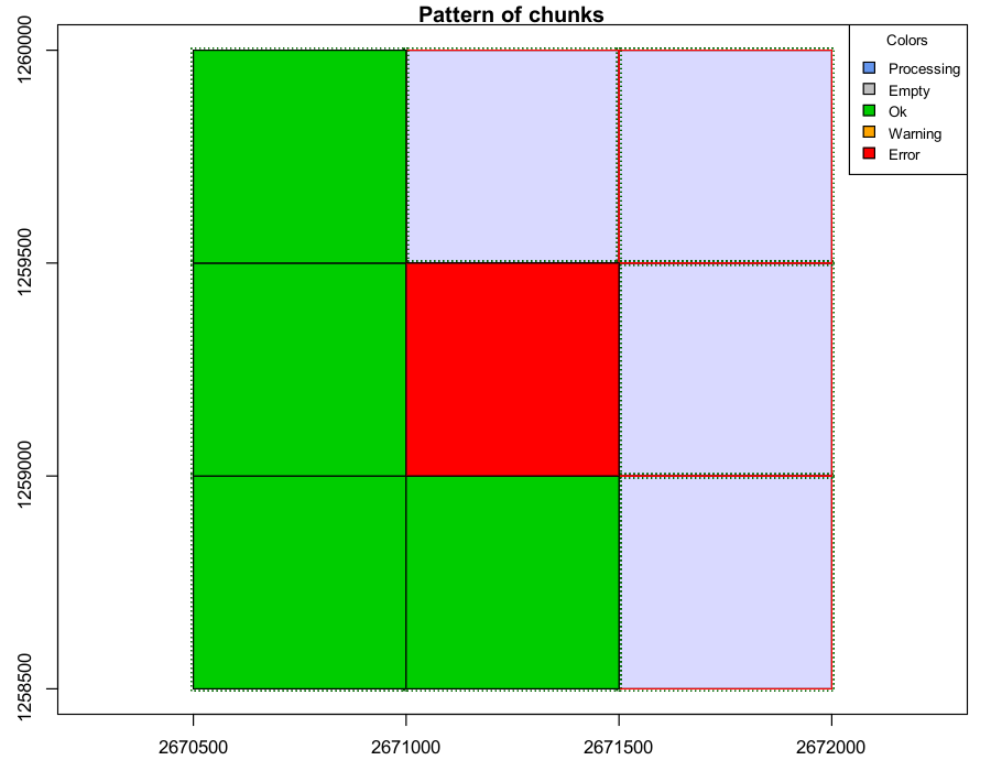
A tile colored in red indicates that the processing failed for that file.
Tip: set opt_stop_early(ctg) <- FALSE to continue processing
File indexing
We can explore indexing of LAScatalog input files for efficient processing.
Indexing generates .lax files associated with each .laz/.las point cloud to speed up processing.
Indexing
The lidR policy has always been: use LAStools and lasindex for spatial indexing. Alternatively there is a hidden function in lidR that users can call (lidR:::catalog_laxindex()).
# check if files have .lax
is.indexed(ctg)
#> [1] FALSE
# generate index files
lidR:::catalog_laxindex(ctg)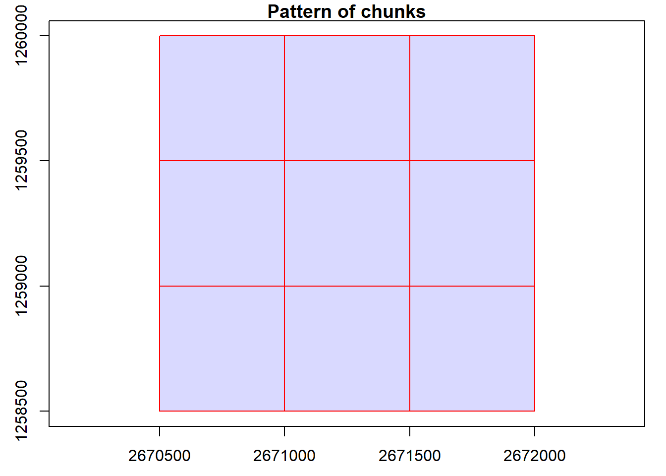
#> Chunk 1 of 9 (11.1%): state ✓
#> Chunk 2 of 9 (22.2%): state ✓
#> Chunk 3 of 9 (33.3%): state ✓
#> Chunk 4 of 9 (44.4%): state ✓
#> Chunk 5 of 9 (55.6%): state ✓
#> Chunk 6 of 9 (66.7%): state ✓
#> Chunk 7 of 9 (77.8%): state ✓
#> Chunk 8 of 9 (88.9%): state ✓
#> Chunk 9 of 9 (100%): state ✓
# check if files have .lax
is.indexed(ctg)
#> [1] TRUE
Generate CHM
Now that we understand how a catalog works, lets apply it to generate some layers.
First create another CHM by rasterizing the point cloud data from the catalog similarly to how we processed a single file.
# Generate CHM
chm <- rasterize_canopy(las = ctg,
                        res = 1,
                        algorithm = p2r(subcircle = 0.15))
#> Chunk 1 of 9 (11.1%): state ✓
#>
Chunk 2 of 9 (22.2%): state ✓
#>
Chunk 3 of 9 (33.3%): state ✓
#>
Chunk 4 of 9 (44.4%): state ✓
#>
Chunk 5 of 9 (55.6%): state ✓
#>
Chunk 6 of 9 (66.7%): state ✓
#>
Chunk 7 of 9 (77.8%): state ✓
#>
Chunk 8 of 9 (88.9%): state ✓
#>
Chunk 9 of 9 (100%): state ✓
#>
plot(chm)
LAScatalog at 1.0m resolution.
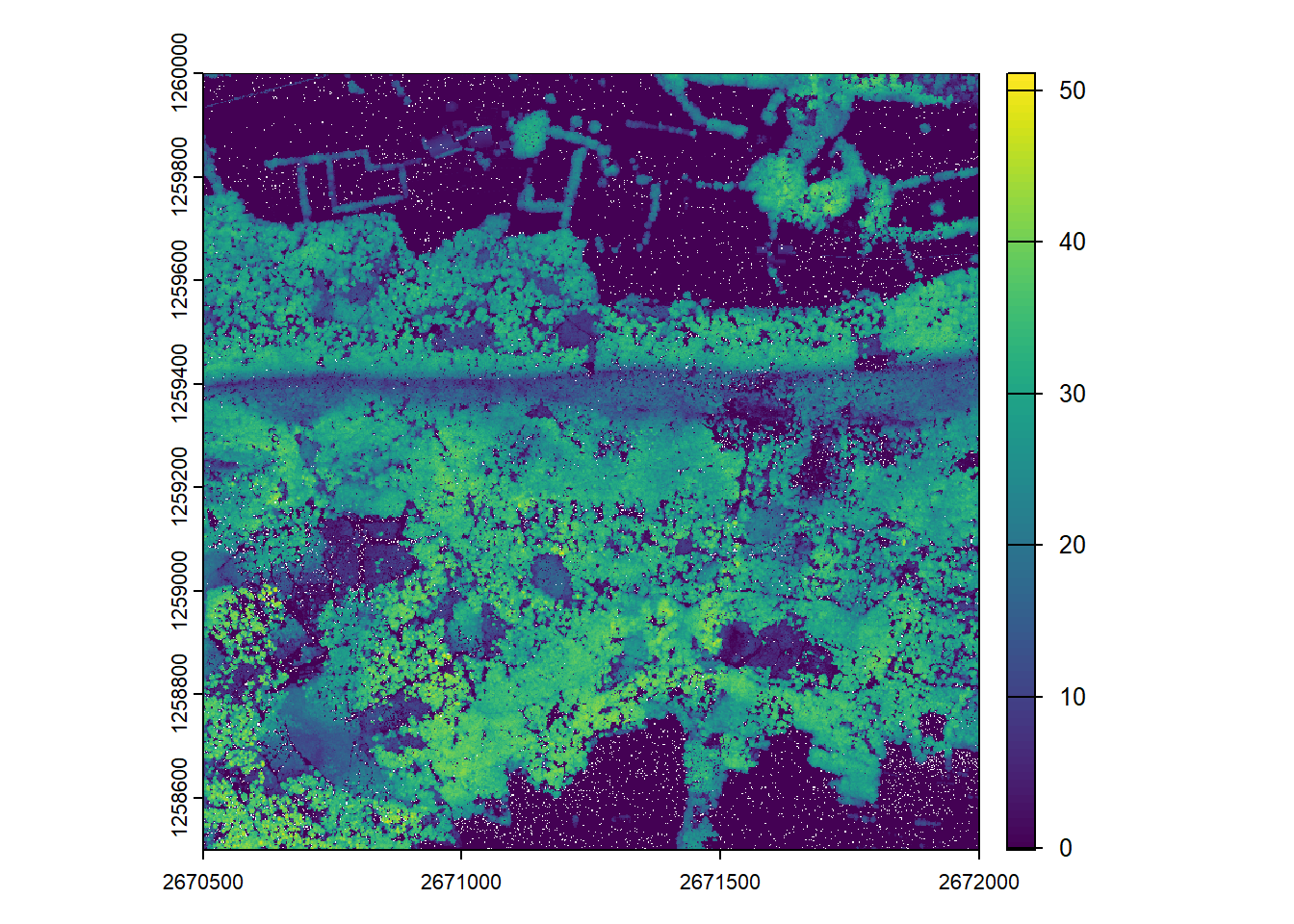
LAScatalog at 1.0m resolution.
Catalog processing options
We can manipulate catalog options to alter processing on-the-fly across all tiles.
# Setting options and re-rasterizing the CHM
opt_filter(ctg) <- "-drop_z_below 0 -drop_z_above 50"
opt_select(ctg) <- "xyz"
chm <- rasterize_canopy(las = ctg, res = 1, algorithm = p2r(subcircle = 0.15))
#> Chunk 1 of 9 (11.1%): state ✓
#>
Chunk 2 of 9 (22.2%): state ✓
#>
Chunk 3 of 9 (33.3%): state ✓
#>
Chunk 4 of 9 (44.4%): state ✓
#>
Chunk 5 of 9 (55.6%): state ✓
#>
Chunk 6 of 9 (66.7%): state ✓
#>
Chunk 7 of 9 (77.8%): state ✓
#>
Chunk 8 of 9 (88.9%): state ✓
#>
Chunk 9 of 9 (100%): state ✓
#>
plot(chm)
LAScatalog after applying filters to drop points below 0m and above 50m.
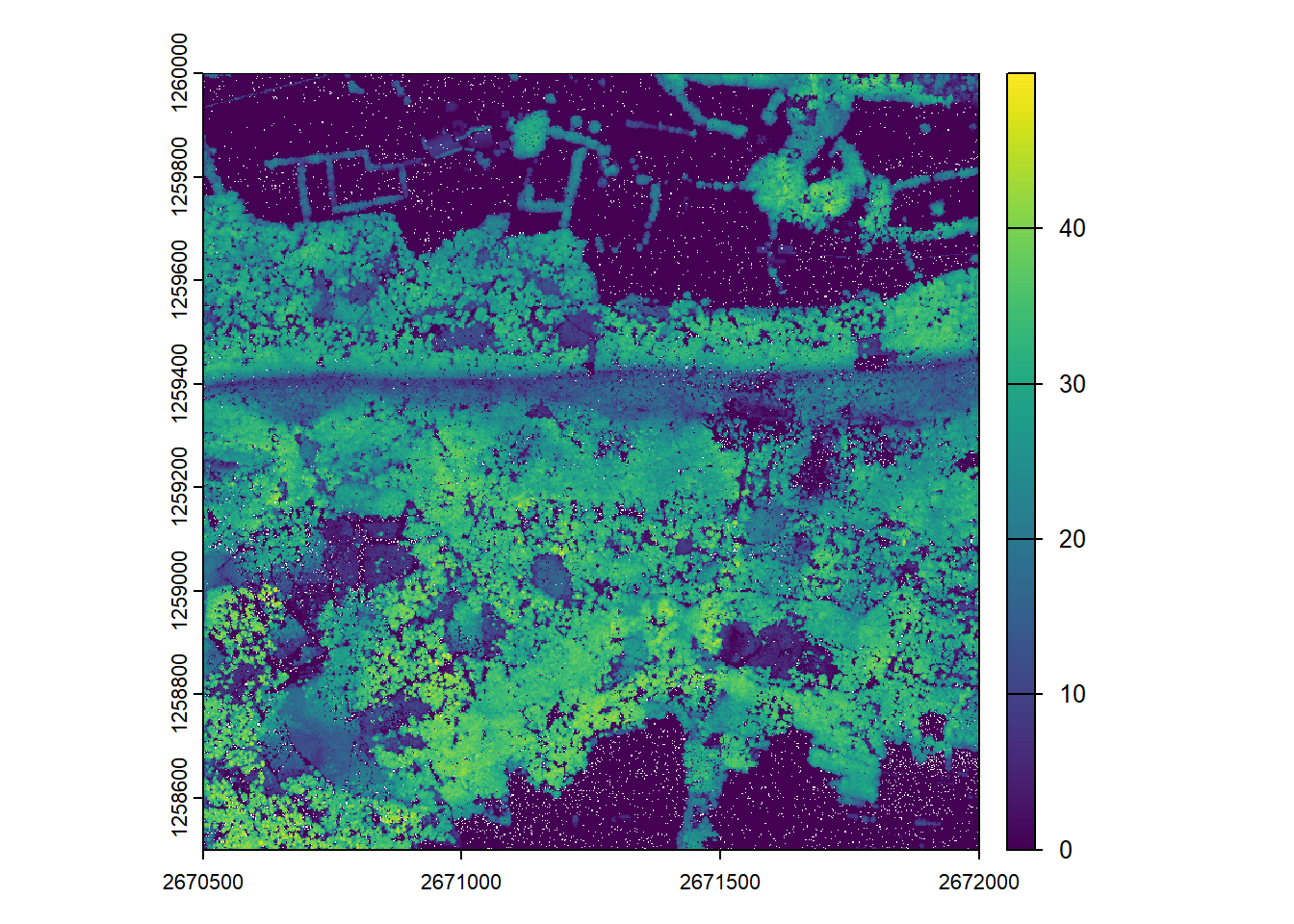
LAScatalog after applying filters to drop points below 0m and above 50m.
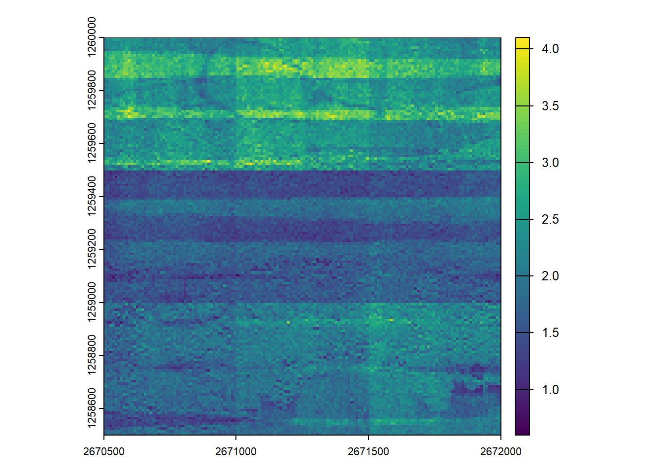
Generate pixel metrics and visualize
We calculate summary metric rasters using the pixel_metrics function and visualize the results.
# Generate pixel-based metrics
max_z <- pixel_metrics(las = ctg, func = ~mean(Z), res = 20)
#> Chunk 1 of 9 (11.1%): state ✓
#>
Chunk 2 of 9 (22.2%): state ✓
#>
Chunk 3 of 9 (33.3%): state ✓
#>
Chunk 4 of 9 (44.4%): state ✓
#>
Chunk 5 of 9 (55.6%): state ✓
#>
Chunk 6 of 9 (66.7%): state ✓
#>
Chunk 7 of 9 (77.8%): state ✓
#>
Chunk 8 of 9 (88.9%): state ✓
#>
Chunk 9 of 9 (100%): state ✓
#>
plot(max_z)
LAScatalog at a 20m resolution.
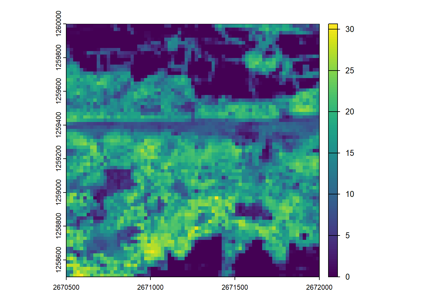
LAScatalog at a 20m resolution.
First returns only
We can adjust the catalog options to calculate metrics based on first returns only.
opt_filter(ctg) <- "-drop_z_below 0 -drop_z_above 50 -keep_first"
max_z <- pixel_metrics(las = ctg, func = ~mean(Z), res = 20)
#> Chunk 1 of 9 (11.1%): state ✓
#>
Chunk 2 of 9 (22.2%): state ✓
#>
Chunk 3 of 9 (33.3%): state ✓
#>
Chunk 4 of 9 (44.4%): state ✓
#>
Chunk 5 of 9 (55.6%): state ✓
#>
Chunk 6 of 9 (66.7%): state ✓
#>
Chunk 7 of 9 (77.8%): state ✓
#>
Chunk 8 of 9 (88.9%): state ✓
#>
Chunk 9 of 9 (100%): state ✓
#>
plot(max_z)
LAScatalog at 20m resolution.
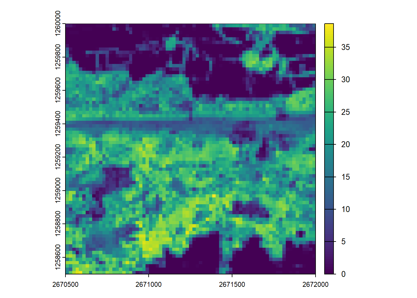
LAScatalog at 20m resolution.
Specifying catalog options
We can define how the LAScatalog should be broken down into chunks for processing. A 10m buffer is added to each chunk to avoid edge artifacts when a function’s calculations depend on neighboring points (also automatically applied by default).
# Specify options
opt_select(ctg) <- "xyz"
opt_chunk_size(ctg) <- 500
opt_chunk_buffer(ctg) <- 10
opt_progress(ctg) <- TRUE

# Visualize and summarize the catalog chunks
plot(ctg, chunk = TRUE)
summary(ctg)
#> class       : LAScatalog (v1.1 format 1)
#> extent      : 2670500, 2672000, 1258500, 1260000 (xmin, xmax, ymin, ymax)
#> coord. ref. : CH1903+ / LV95
#> area        : 2.25 km²
#> points      : 11.25 million points
#> type        : airborne
#> density     : 5 points/m²
#> density     : 2 pulses/m²
#> num. files  : 9
#> proc. opt.  : buffer: 10 | chunk: 500
#> input opt.  : select: xyz | filter: -drop_z_below 0 -drop_z_above 50 -keep_first
#> output opt. : in memory | w2w guaranteed | merging enabled
#> drivers     :
#>  - Raster : format = GTiff  NAflag = -999999
#>  - stars : NA_value = -999999
#>  - Spatial : overwrite = FALSE
#>  - SpatRaster : overwrite = FALSE  NAflag = -999999
#>  - SpatVector : overwrite = FALSE
#>  - LAS : no parameter
#>  - sf : quiet = TRUE
#>  - data.frame : no parameter
LAScatalog processing chunks, with a size of 500m (red solid lines) and a 10m buffer (green dashed lines).
Parallel computing
In this section, we explore parallel computing using the lidR package.
Parallel computing can apply the
Note
Resource Considerations for Parallel Processing:
Be mindful of your system’s resources. Parallel processing loads multiple tiles into memory (RAM) simultaneously. The required memory depends on the number of workers (cores), the point density and size of your tiles, and the complexity of the function being applied. If you encounter memory-related errors, try reducing the number of workers.
Run parallel::detectCores() to see avaliable workers - limit your use to a fraction of available cores as other processes on your machine require computation.
Load future library
Firstly, we load the future library to enable parallel processing.
library(future)Single core processing
To establish a baseline, we generate a point density raster using a single processing core.
plan(sequential) from future ensures that the code runs sequentially, not in parallel.
# Process on single core
plan(sequential)

# Generate a point density raster (points per square metre)
dens_seq <- rasterize_density(ctg, res = 10)
#> Chunk 1 of 9 (11.1%): state ✓
#>

Chunk 2 of 9 (22.2%): state ✓
#>

Chunk 3 of 9 (33.3%): state ✓
#>

Chunk 4 of 9 (44.4%): state ✓
#>

Chunk 5 of 9 (55.6%): state ✓
#>

Chunk 6 of 9 (66.7%): state ✓
#>

Chunk 7 of 9 (77.8%): state ✓
#>

Chunk 8 of 9 (88.9%): state ✓
#>

Chunk 9 of 9 (100%): state ✓
#>


plot(dens_seq)

Parallel processing
Now, we’ll perform the same operation but leverage multiple cores.
In calling plan(multisession, workers = 3L) from future, lidR will automatically distribute the processing chunks across three CPU cores (workers).
The result should be identical to the single-core version, and should be faster than single-core systems.
# Process on multi-core with three workers
plan(multisession, workers = 3L)

# Generate the same density raster, but in parallel
dens_par <- rasterize_density(ctg, res = 10)
#> Chunk 1 of 9 (11.1%): state ✓
#>

Chunk 2 of 9 (22.2%): state ✓
#>

Chunk 3 of 9 (33.3%): state ✓
#>

Chunk 4 of 9 (44.4%): state ✓
#>

Chunk 5 of 9 (55.6%): state ✓
#>

Chunk 6 of 9 (66.7%): state ✓
#>

Chunk 7 of 9 (77.8%): state ✓
#>

Chunk 8 of 9 (88.9%): state ✓
#>

Chunk 9 of 9 (100%): state ✓
#>


plot(dens_par)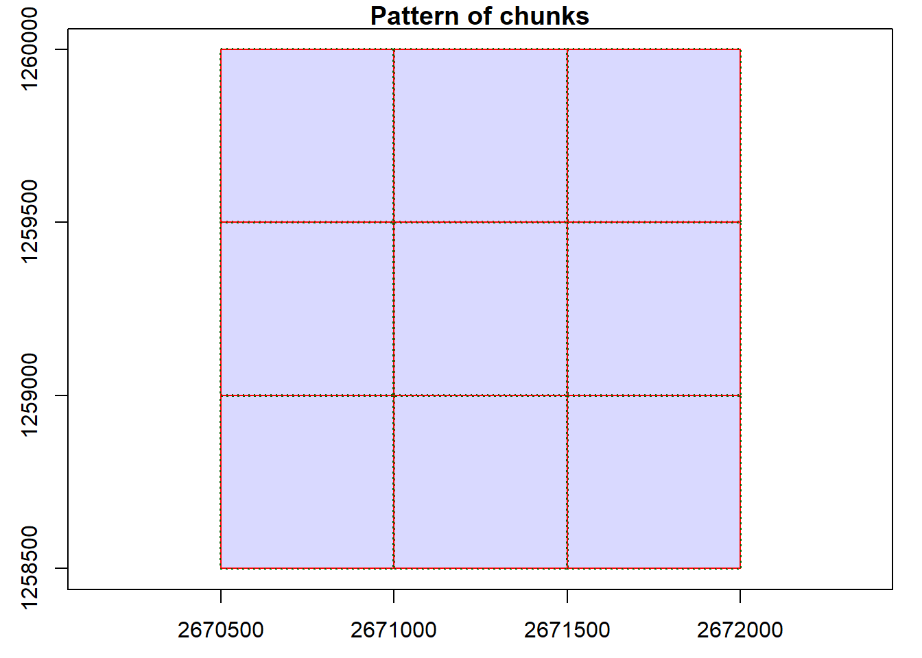
Revert to single core
It is good practice to always return the plan(sequential) after a parallel task is complete to avoid unintended parallel execution in later code.
# Back to single core
plan(sequential)
Conclusion
This concludes the tutorial on basic usage, catalog validation, indexing, CHM generation, metric generation, and parallel computing to generate point density rasters using the lidR and future packages in R.
Exercises
Using:
ctg <- readLAScatalog(folder = "data/ctg_norm")
E1.
Calculate a set of metrics from the lidRmetrics package on the catalogue (voxel metrics will take too long)
Using:
ctg <- readLAScatalog(folder = "data/ctg_class")
E2.
Read in the non-normalized las catalog filtering the point cloud to only include first returns.
E3.
Generate a DTM at 1m spatial resolution for the provided catalog with only first returns.
Tip
The Multiple Returns and Canopy Penetration This exercise highlights a critical and unique capability of Airborne Laser Scanning (ALS).
Unlike methods based on imagery like Digital Aerial Photogrammetry (DAP), map the visible surface, lidar pulses can penetrate through gaps in the vegetation generating multiple returns each. This allows us to map the ground surface even under dense forest cover, which is essential for creating accurate Digital Terrain Models (DTMs).