# Clear environment
rm(list = ls(globalenv()))

# Load packages
library(lidR)
library(terra)Canopy Height Models
Relevant Resources
Overview
This code demonstrates the creation of a Canopy Height Model (CHM). Similar to the DTM, a CHM is a rasterized summary of the upper-most surface of the height normalized lidar point cloud. Often this is simply generated as maximum height for each cell. CHMs often serve as fundamental layers for vegetation and biodiversity related applications.
We present different algorithms for generating CHMs and provide options for adjusting resolution and filling empty pixels.
Environment
Data Preprocessing
Once again we load the lidar in to memory with readLAS. this time however, we sample points randomly to decimate the point cloud and simulate lower density lidar data using decimate_points().
The sampling/return density of your point cloud (particularly those originating from the canopy surface for a CHM) dictates the lowest acceptable spatial resolution.
# Load lidar data and reduce point density
las <- readLAS(files = "data/zrh_norm.laz")
# Density of the data is reduced from 20 points/m² to 10 points/m² for example purposes
las <- decimate_points(las, random(density = 10))
# Visualize the lidar point cloud
plot(las)
Point-to-Raster Based Algorithm
First we apply a simple method for generating Canopy Height Models (CHMs).
Below, the rasterize_canopy() function with the p2r() algorithm assigns the elevation of the highest point within each 2m grid cell to a corresponding pixel. The resulting CHM is then visualized using the plot() function.
# Generate the CHM using a simple point-to-raster based algorithm
chm <- rasterize_canopy(las = las, res = 2, algorithm = p2r())

# Visualize the CHM
plot(chm)
p2r) algorithm.
Next, by increasing the resolution of the CHM to 1m (reducing the grid cell size), we get a more detailed representation of the canopy, but also have more empty pixels.
# Make spatial resolution 1 m
chm <- rasterize_canopy(las = las, res = 1, algorithm = p2r())
plot(chm)
p2r algorithm, showing more detail and some empty pixels.
Further increasing to 0.5m causes more empty pixels where no valid points are present. (see tiny white dots on CHM)
# Using the 'subcircle' option turns each point into a disc of 8 points with a radius r
chm <- rasterize_canopy(las = las, res = 0.5, algorithm = p2r(subcircle = 0.15))
plot(chm)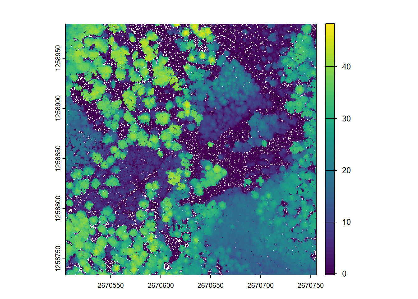
p2r algorithm with the subcircle option to fill gaps.
The rasterize_canopy() function with the p2r() algorithm allows the use of the subcircle option, which turns each lidar point into a disc of 8 points with a specified radius. This can help to capture more fine-grained canopy details, especially from lower density point clouds, resulting in a complete CHM.
Increasing the subcircle radius may not necessarily result in meaningful CHMs, as it could lead to over-smoothing or loss of important canopy information.
# Increasing the subcircle radius, but it may not have meaningful results
chm <- rasterize_canopy(las = las, res = 0.5, algorithm = p2r(subcircle = 0.8))
plot(chm)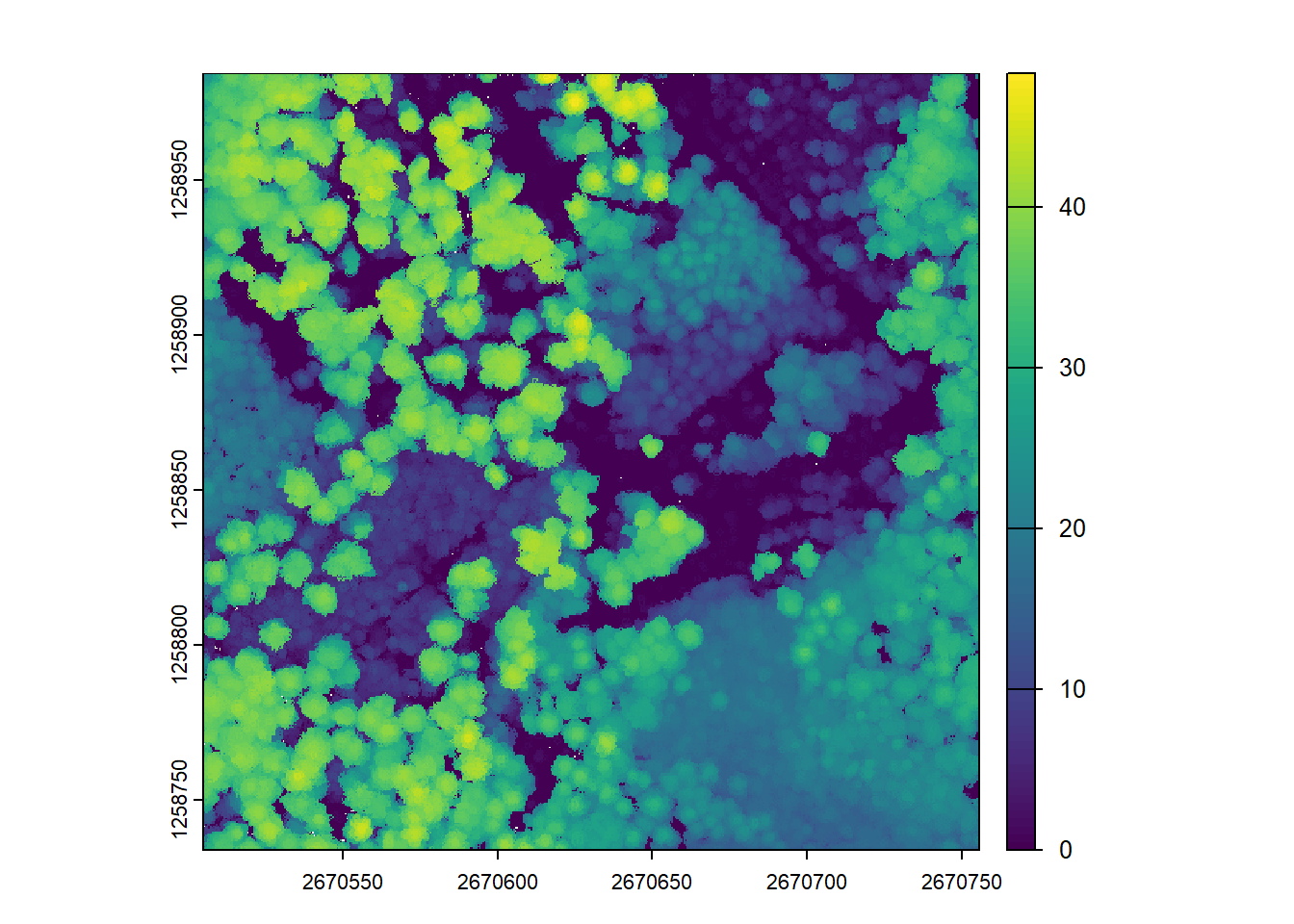
subcircle radius, with potential over-smoothing.
The p2r() algorithm also allows filling empty pixels using TIN (Triangulated Irregular Network) interpolation, which can help in areas with sparse lidar points to obtain a smoother CHM.
# We can fill empty pixels using TIN interpolation
chm <- rasterize_canopy(las = las, res = 0.5, algorithm = p2r(subcircle = 0.0, na.fill = tin()))
plot(chm)
Triangulation Based Pitfree Algorithm
The rasterize_canopy function can also use the Khosravipour et al. 2014 pitfree() algorithm with specified height thresholds and a maximum edge length to generate a CHM. This algorithm aims to correct depressions in the CHM surface, especially designed to prevent gaps in CHMs from low density lidar.
Pit-free algorithm
Check out Khosravipour et al. 2014 to see the original implementation of the algorithm!
# Using the Khosravipour et al. 2014 pit-free algorithm with specified thresholds and maximum edge length
thresholds <- c(0, 5, 10, 20, 25, 30)
max_edge <- c(0, 1.35)
chm <- rasterize_canopy(las = las, res = 0.5, algorithm = pitfree(thresholds, max_edge))
plot(chm)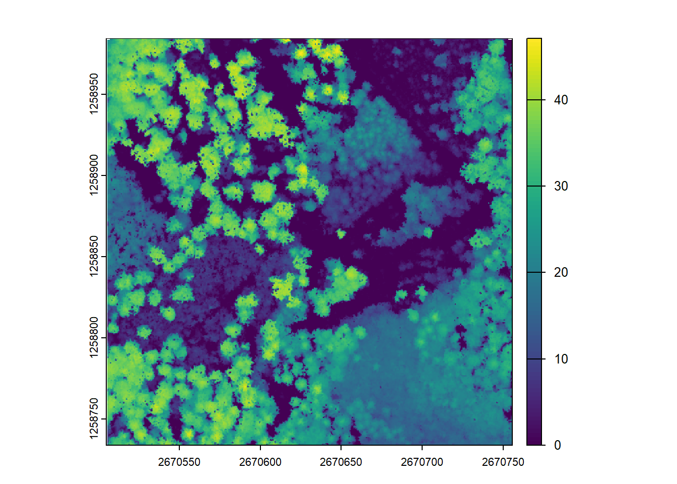
pitfree algorithm by Khosravipour et al. (2014).
The subcircle option can also be used with the pitfree() algorithm to create finer spatial resolution CHMs with subcircles for each lidar point, similar to the point-to-raster based algorithm.
# Using the 'subcircle' option with the pit-free algorithm
chm <- rasterize_canopy(las = las, res = 0.25, algorithm = pitfree(thresholds, max_edge, 0.1))
plot(chm)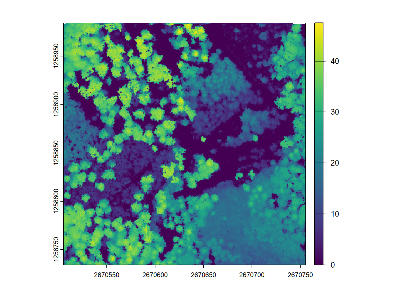
pitfree algorithm combined with the subcircle option for finer detail.
Post-Processing
CHMs can be post-processed by smoothing or other manipulations. Here, we demonstrate post-processing using the terra::focal() function for average smoothing within a 3x3 moving window.
# Post-process the CHM using the 'terra' package and focal() function for smoothing
ker <- matrix(1, 3, 3)
schm <- terra::focal(chm, w = ker, fun = mean, na.rm = TRUE)

# Visualize the smoothed CHM
plot(schm)
pitfree CHM after post-processing with a 3x3 mean focal filter for smoothing.
Exercises
E1.
Using the p2r() and pitfree() (defining your own arguments) create two CHMs with the same resolution and plot them. What differences do you notice?
E2.
Using terra::focal() with the w = matrix(1, 5, 5) and fun = max, plot a manipulated CHM using one of the CHMs you previously generated.
E3.
Create a 10 m CHM using a algorithm of your choice. Would this information still be useful at this scale?
Conclusion
This tutorial covered different algorithms for generating Canopy Height Models (CHMs) from lidar data using the lidR package in R. It includes point-to-raster-based algorithms and triangulation-based algorithms, as well as post-processing using the terra package.