# Clear environment
rm(list = ls(globalenv()))

# Load package
library(lidR)Read/Plot/Query
Relevant Resources
Overview
Welcome to this lidar processing tutorial using R and the lidR package! In this tutorial, you will learn how to read, visualize, and query lidar data. We’ll explore basic information about a lidar file including the header and data frame as well as visualize point clouds using different colour schemes based on attributes with plot(). We’ll use the select argument in readLAS() to load specific attributes and the filter argument to only load points of interest or apply transformations on-the-fly.
Let’s get started with processing lidar data efficiently using lidR and R! Happy learning!
Environment
We start each page by loading the necessary packages, clearing our current environment, and specifying that some warnings be turned off to make our outputs clearer. We will do this for each section in the tutorial.
Basic Usage
Load and Inspect lidar Data
Load the lidar point cloud data from a LAS file using the readLAS() function. The data is stored in the las object. We can inspect the header information and attributes of the las object by calling the object.
# Load the sample point cloud
las <- readLAS(files = "data/zrh_norm.laz")
# Inspect header information and print a summary
las
#> class        : LAS (v1.1 format 1)
#> memory       : 67.8 Mb
#> extent       : 2670505, 2670755, 1258734, 1258984 (xmin, xmax, ymin, ymax)
#> coord. ref.  : CH1903+ / LV95
#> area         : 63504 m²
#> points       : 1.27 million points
#> type         : airborne
#> density      : 20 points/m²
#> density      : 7.43 pulses/m²

# Check the file size of the loaded lidar data
format(object.size(las), "Mb")
#> [1] "96.9 Mb"
Visualizing lidar Data
We can visualize the lidar data using the plot() function. We have several options to control the colours in the plot, such as selecting specific attributes from the data to be mapped.
plot() background colour
Set the background of plots to white using plot(las, bg = "white"). To keep the website code clean I’ve omitted this from examples.
plot(las)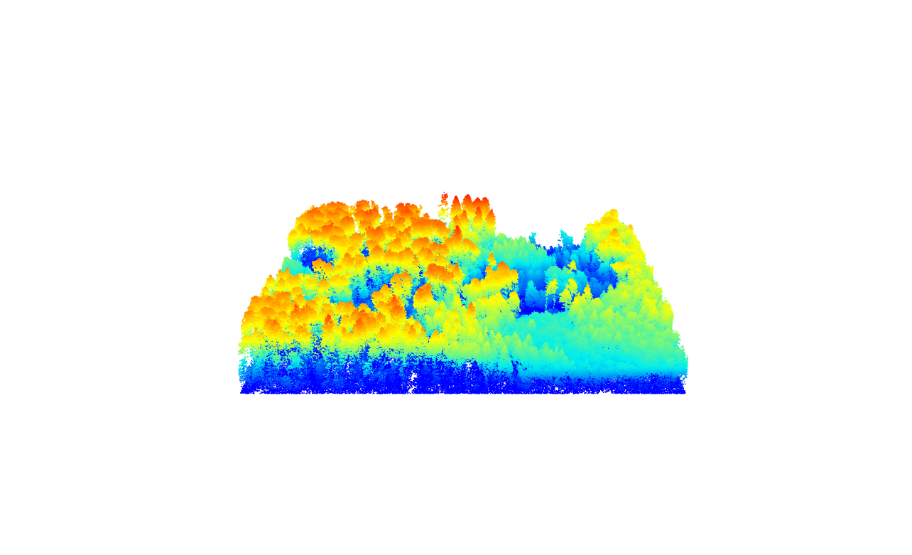
Point Classification
Lidar systems and pre-processing attribute point clouds with additional attributes beyond just X, Y and Z coordinates.
For instance, points are typically assigned Classification values to differentiate surfaces. This is often already done by the data provider or through user applied algorithms to classify for example noise and ground points. The meaning of these ID values depends on the LAS file version and source.
Note
LAS Standard Point classification is now standardized by the American Society for Photogrammetry and Remote Sensing (ASPRS). For a complete list of classes, refer to the LAS 1.4 specification (R15).
Our example ALS dataset, collected in 2014 over Zürich uses an older LAS 1.1 standard. Its classification codes are interpreted as follows:
| Class Code | Meaning | Interpretation | Number of points |
|---|---|---|---|
| 2 | Ground | The bare earth surface. | |
| 3/4/5 | Low/Medium/High Vegetation | Vegetation under 1 meter. | |
| 7 | Noise | Erroneous points, likely below ground or outliers above ground. | 87 |
| 12 | Overlap Points | Points assigned to overlapping flight lines. | |
plot(las, color = "Classification")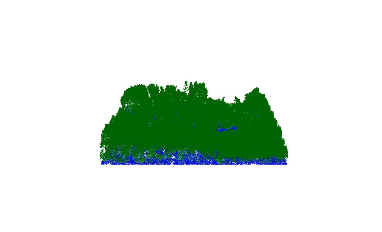
Lidar point clouds record Return Intensity information; representing the strength of the returning signal. This attribute varies widely depending on sensor/acquisition characteristics can be useful in biodiversity mapping.
plot(las, color = "Intensity")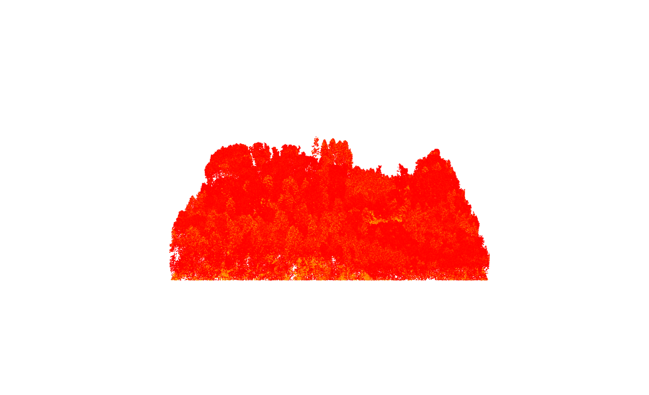
Laser scanning systems record the scan angle of each pulse and attribute this information to the point cloud as ScanAngleRank.
plot(las, color = "ScanAngleRank")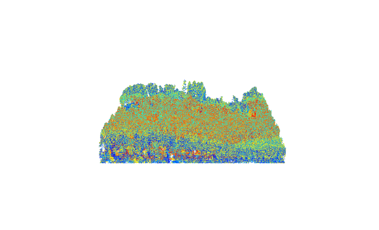
Filtering Dataset
Often we do not need the entire set of points or attributes (columns) loaded in memory for our analysis. We can use Classification as well as other attributes to pre-filter point clouds before further processing.
There are two key was in lidR to achieve this.
Filtering points on-the-fly (efficient)
First, we load subsets of the lidar points based on certain criteria using the filter argument in directly in readLAS().
The filter argument in readLAS() can be useful for tasks such as filtering specific classifications, to isolate ground, remove noise, etc…
# Load point cloud keeping only Classification 2 (ground returns)
las <- readLAS(files = "data/zrh_class.laz", filter = "-keep_class 2")
Visualize the first return filtered point cloud using the plot() function.
plot(las)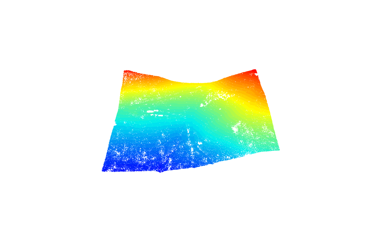
-keep_class 2.
Each lidar pulse can record multiple discrete returns (points).
Here we use a filter during readLAS to subset only first returns.
# Load only the first return points
las <- readLAS(files = "data/zrh_norm.laz", filter = "-keep_first")
# Inspect the loaded points
las
#> class : LAS (v1.1 format 1)
#> memory : 25.2 Mb
#> extent : 2670505, 2670755, 1258734, 1258984 (xmin, xmax, ymin, ymax)
#> coord. ref. : CH1903+ / LV95
#> area : 63476 m²
#> points : 471.7 thousand points
#> type : airborne
#> density : 7.43 points/m²
#> density : 7.43 pulses/m²
# Check the memory size after loading only the filtered points
format(object.size(las), "Mb")
#> [1] "36 Mb"Visualize the first return filtered point cloud using the plot() function.
plot(las)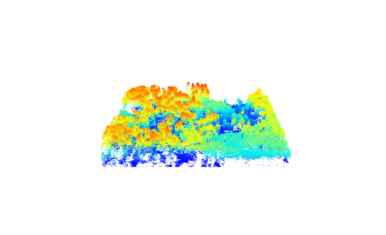
-keep_first.
The readLAS() function also allows us to select specific attributes (columns) to be loaded into memory. This is useful to reduce memory requirements when working with large lidar datasets.
# Load only the xyz coordinates (X, Y, Z) and ignore other attributes
las <- readLAS(files = "data/zrh_norm.laz", select = "xyz")
# Inspect the loaded attributes
las@data
#> X Y Z
#> <num> <num> <num>
#> 1: 2670506 1258984 18.57
#> 2: 2670506 1258984 23.27
#> 3: 2670506 1258984 20.64
#> 4: 2670507 1258984 0.00
#> 5: 2670505 1258983 0.00
#> ---
#> 1270076: 2670754 1258736 17.38
#> 1270077: 2670754 1258736 17.72
#> 1270078: 2670754 1258735 13.45
#> 1270079: 2670754 1258735 16.41
#> 1270080: 2670754 1258734 15.43
# Check the memory size (much smaller)
format(object.size(las), "Mb")
#> [1] "29.1 Mb"
See all
readLAS pre-built filters
run readLAS(filter = "-help") for a full list of these filters.
Filtering Points using filter_poi()
Alternatively LASobjects loaded into memory with readLAS() can be filtered immediately using the filter_poi() function. These filters can be custom made by combining boolean operators (==, !=, >, <, &, |, etc…) with point cloud attributes to formulate logical statements. Statements are applied to points to assign TRUE (kept) or FALSE (filtered out) values.
# Load the lidar file with all the all attributes
las <- readLAS(files = "data/zrh_class.laz")
# Filter points with Classification == 2
class_2 <- filter_poi(las = las, Classification == 2L)
# Combine queries to filter points with Classification 2 and ReturnNumber == 1
first_returns <- filter_poi(las = las, Classification == 2L & ReturnNumber == 1L)plot(class_2)
filter_poi().
plot(first_returns)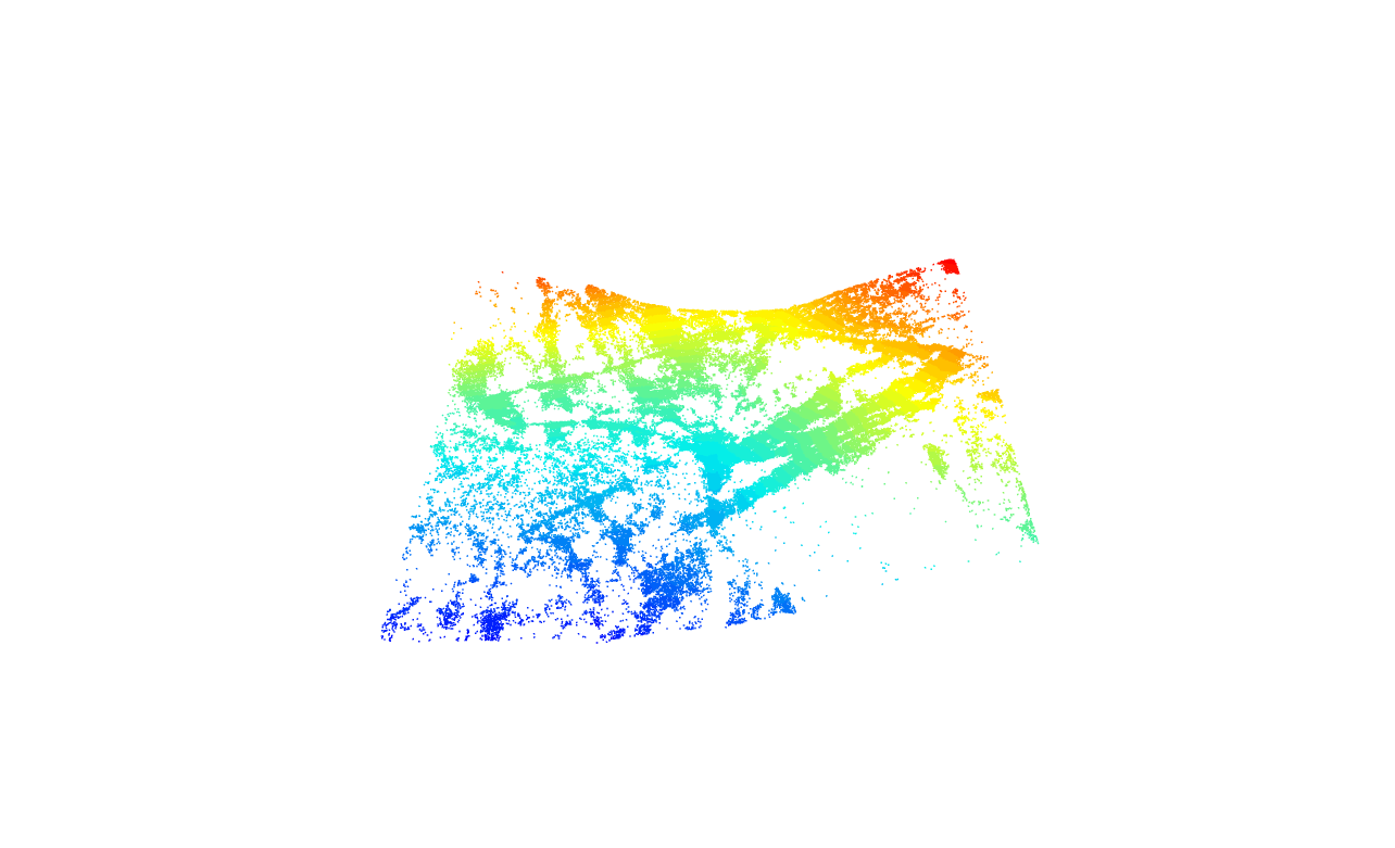
filter_poi().
Exercises and Questions
Using:
las <- readLAS(files = "data/zrh_norm.laz")E1.
Using the plot() function plot the point cloud with a different attribute that has not been done yet
Try adding axis = TRUE, legend = TRUE to your plot argument plot(las, axis = TRUE, legend = TRUE)
E2.
Create a filtered las object of returns that have an Intensity greater that 50, and plot it.
E3.
Read in the las file with only xyz and intensity only. Hint go to the lidRbook section to find out how to do this
Conclusion
This concludes our tutorial on the basic usage of the lidR package in R for processing and analyzing lidar data. We covered loading lidar data, inspecting and visualizing the data, selecting specific attributes, and filtering points of interest.