# Clear environment
rm(list = ls(globalenv()))

# Load packages
library(lidR)Digital Terrain Models
Relevant resources
Overview
Airborne Laser Scanning has for decades been used to generate detailed models of terrain based on lidar measurements. Lidar’s ability to produce consistent wall-to-wall ground measurements, even when obscured by vegetation is a critical advantage of the technology in environmental mapping.
Digital Terrain Models (DTMs) are gridded (raster) surfaces generated at a given spatial resolution with an interpolation method that populates each cell with an elevation value.
This tutorial explores the creation of DTMs from lidar data. It demonstrates two algorithms for DTM generation: ground point triangulation, and inverse-distance weighting. Additionally, the tutorial showcases DTM-based normalization and point-based normalization, accompanied by exercises for hands-on practice.
Environment
DTM (Digital Terrain Model)
In this section, we’ll generate a Digital Terrain Model (DTM) from lidar data using two different algorithms: tin() and knnidw().
Data Preprocessing
# Load lidar data where points are already pre-classified
las <- readLAS(files = "data/zrh_class.laz")
Visualizing Lidar Data
We start by visualizing the entire lidar point cloud to get an initial overview.
plot(las)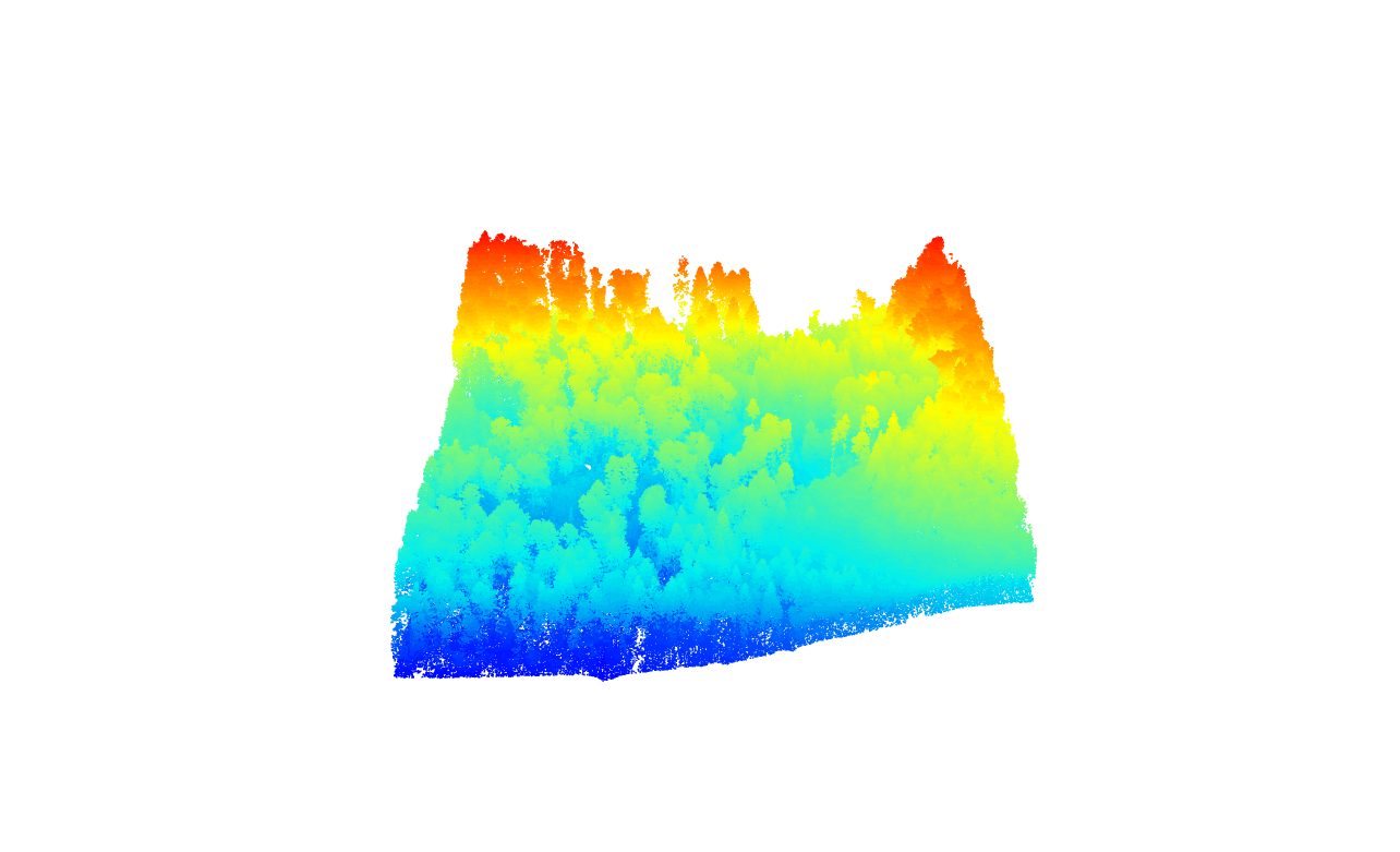
Visualizing the Lidar data again, this time to distinguish ground points (blue) more effectively.
plot(las, color = "Classification")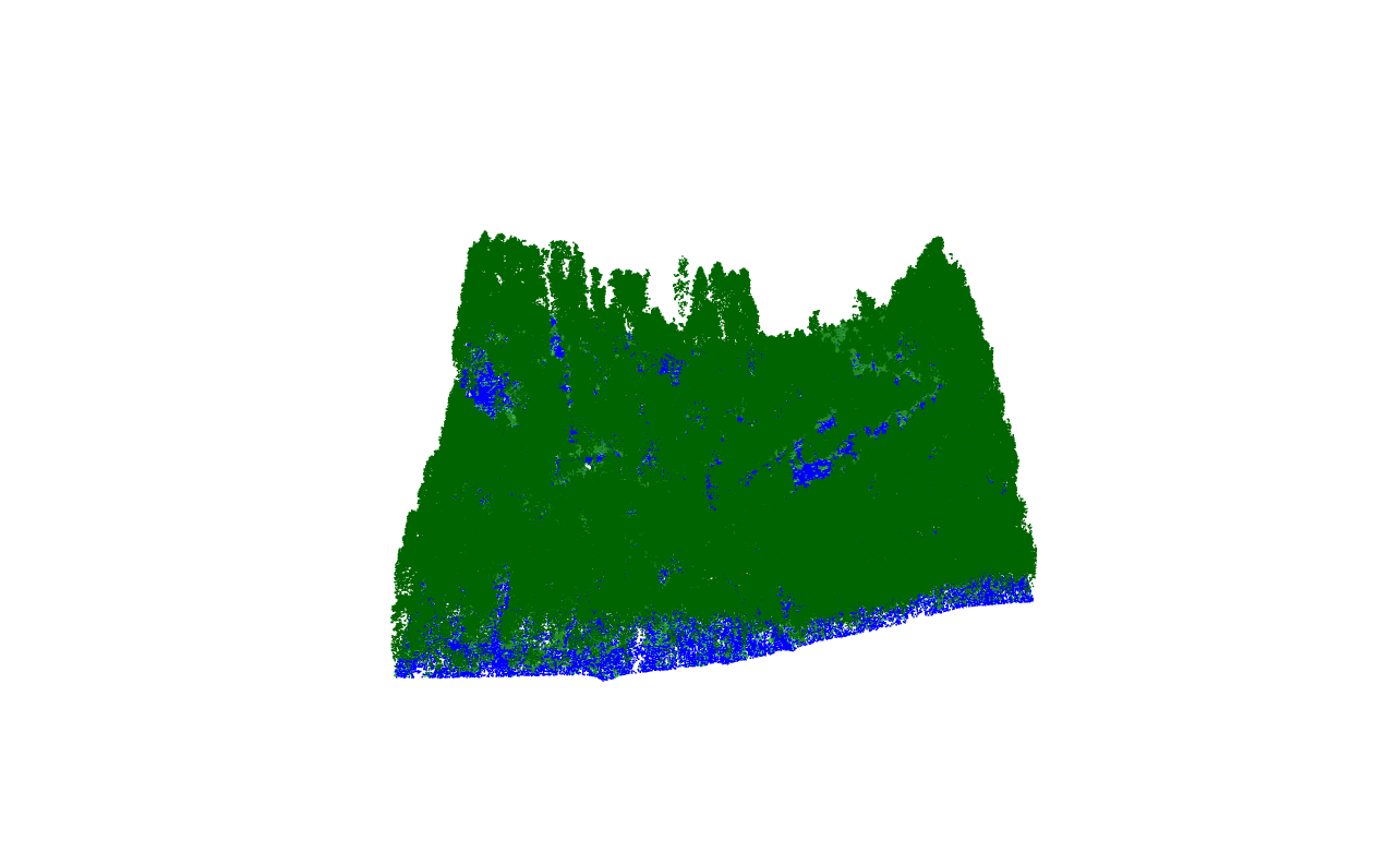
Triangulation Algorithm - tin()
We create a DTM using the tin() algorithm with a resolution of 1 meter.
# Generate a DTM using the TIN (Triangulated Irregular Network) algorithm
dtm_tin <- rasterize_terrain(las = las, res = 1, algorithm = tin())
Degenerated points
You may receive a warning about degenerated points when creating a DTM. A degenerated point in lidar data refers to a point with identical XY(Z) coordinates as another point. This means two or more points occupy exactly the same location in XY/3D space. Degenerated points can cause issues in tasks like creating a digital terrain model, as they don’t add new information and can lead to inconsistencies. Identifying and handling degenerated points appropriately is crucial for accurate and meaningful results.
Visualizing DTM in 3D
To better conceptualize the terrain, we visualize the generated DTM in a 3D plot.
# Visualize the DTM in 3D
plot_dtm3d(dtm_tin)
tin() algorithm.
Visualizing DTM with Lidar Point Cloud
We overlay the DTM on the lidar data (non-ground points only) for a more comprehensive view of the terrain.
# Filter for non-ground points to show dtm better
las_ng <- filter_poi(las = las, Classification != 2L)

# Visualize the lidar data with the overlaid DTM in 3D
x <- plot(las_ng, bg = "white")
add_dtm3d(x, dtm_tin, bg = "white")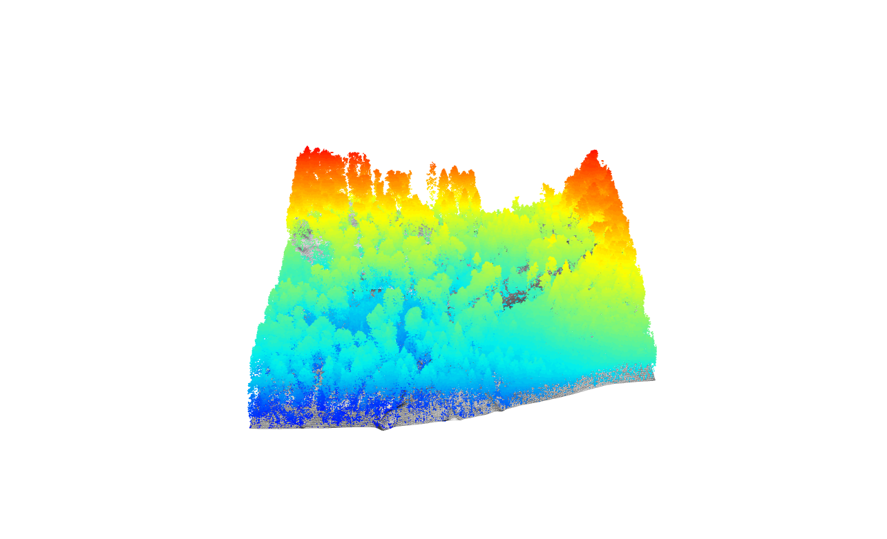
tin() generated DTM overlaid with the non-ground lidar points.
Inverse-Distance Weighting (IDW) Algorithm - knnidw()
Next, we generate a DTM using the IDW algorithm to compare results with the TIN-based DTM.
# Generate a DTM using the IDW (Inverse-Distance Weighting) algorithm
dtm_idw <- rasterize_terrain(las = las, res = 1, algorithm = knnidw())
Visualizing IDW-based DTM in 3D
We visualize the DTM generated using the IDW algorithm in a 3D plot.
# Visualize the IDW-based DTM in 3D
plot_dtm3d(dtm_idw)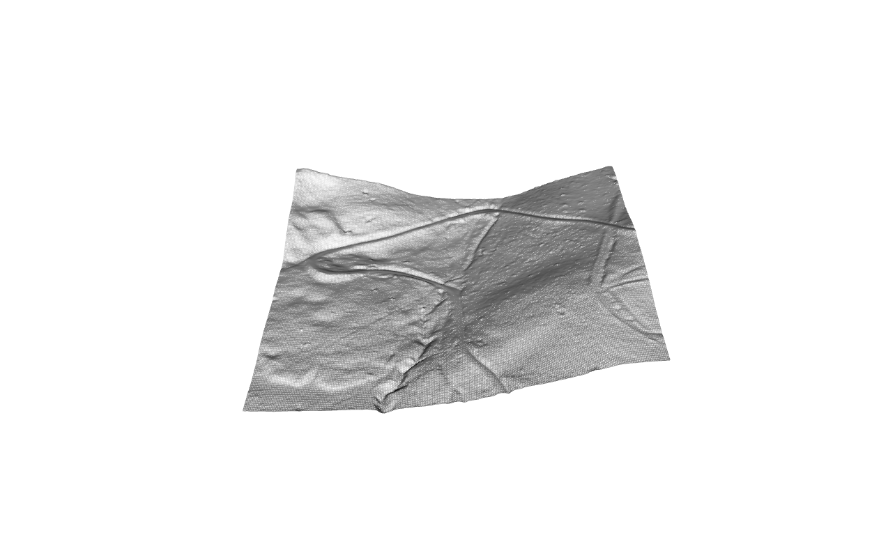
knnidw() algorithm.
Height Normalization
Height normalization is applied by subtracting terrain height from return heights above the ground level. This serves to remove distortion from topography and isolate vegetation structure. In doing so elevation (Z coordinates) of each return is converted from height above some reference surface; such as sea level (mASL) to above ground (mAGL)
Normalization is a critical pre-processing step that enables the signal of vegetation structure to be isolated and mapped.
We’ll perform height normalization of lidar data using both DTM-based and point-based normalization methods.
p_las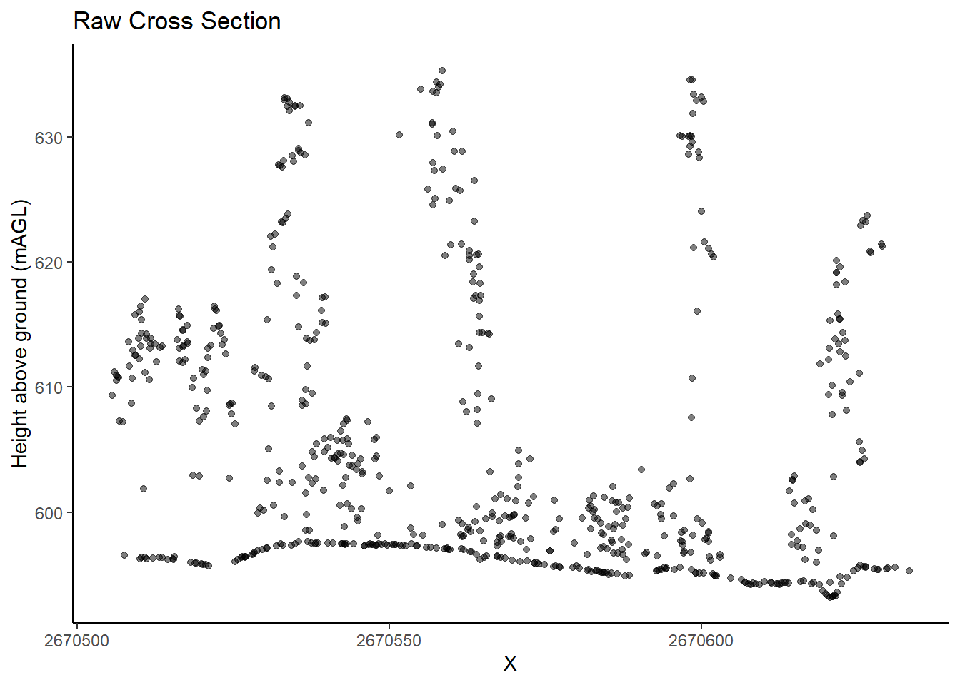
p_norm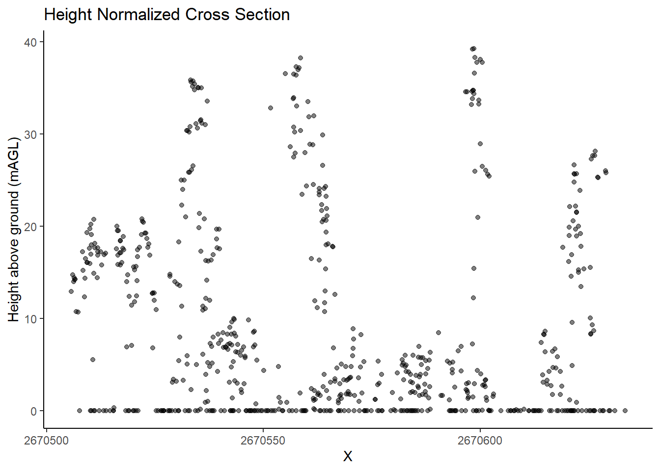
DTM-based Normalization
First, we perform DTM-based normalization on the lidar data using the previously generated DTM.
# Normalize the lidar data using DTM-based normalization
nlas_dtm <- normalize_height(las = las, algorithm = dtm_tin)
Visualizing Normalized Lidar Data
We visualize the normalized lidar data, illustrating heights relative to the DTM (mAGL).
# Visualize the normalized lidar data
plot(nlas_dtm)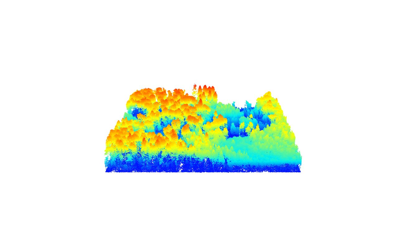
DTM-based Normalization with TIN Algorithm
We perform DTM-based normalization on the lidar data using the TIN algorithm. Rather than specifying a resolution for an interpolated DTM a triangular irregular network (TIN) will be directly fit to ground returns (on-the-fly) and used to normalize points elevations.
# Normalize the lidar data using DTM-based normalization with TIN algorithm
nlas_tin <- normalize_height(las = las, algorithm = tin())
Visualizing Normalized Lidar Data with TIN
We visualize the normalized lidar data using the TIN algorithm, showing heights relative to the DTM.
# Visualize the normalized lidar data using the TIN algorithm
plot(nlas_tin, bg = "white")
Exercises
E1.
Compute two DTMs for this point cloud with differing spatial resolutions, plot both
E2.
Now use the plot_dtm3d() function to visualize and move around your newly created DTMs
Conclusion
This tutorial covered the creation of Digital Terrain Models (DTMs) from lidar data using different algorithms and explored height normalization techniques. The exercises provided hands-on opportunities to apply these concepts, enhancing understanding and practical skills.