Excercise Solutions

Resources

Code

1-LAS

# Load packages
library(sf)
library(terra)
library(lidR)
library(lidRmetrics)

E1.

Using the plot() function plot the point cloud with a different attribute that has not been done yet

Try adding axis = TRUE, legend = TRUE to your plot argument plot(las, axis = TRUE, legend = TRUE)

Code

las <- readLAS(files = "data/zrh_norm.laz")

Code

plot(las, color = "ReturnNumber", axis = TRUE, legend = TRUE)

E2.

Create a filtered las object of returns that have an Intensity greater that 50, and plot it.

Code

las <- readLAS(files = "data/zrh_norm.laz")

Code

i_50 <- filter_poi(las = las, Intensity > 50)
plot(i_50)

E3.

Read in the las file with only xyz and intensity only. Hint go to the lidRbook section to find out how to do this.

Code

las <- readLAS(files = "data/zrh_norm.laz", select = "xyzi")

2-DTM

E1.

Compute two DTMs for this point cloud with differing spatial resolutions, plot both e.g. `plot(dtm1)

Code

las <- readLAS(files = "data/zrh_class.laz")

Code

dtm_5 <- rasterize_terrain(las=las, res=5, algorithm=tin())
dtm_10 <- rasterize_terrain(las=las, res=10, algorithm=tin())
plot(dtm_5)

Code

plot(dtm_10)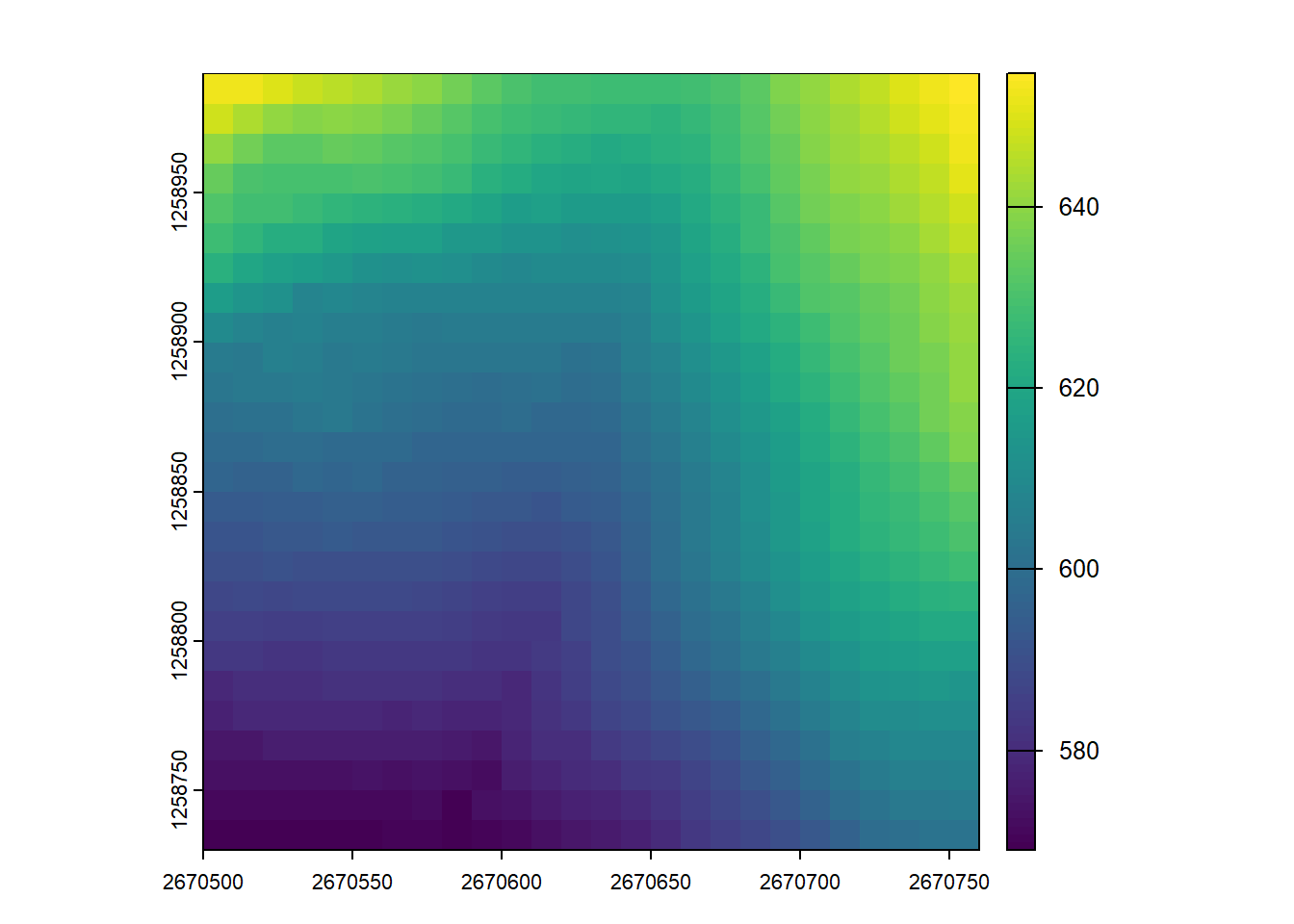

E2.

Now use the plot_dtm3d() function to visualize and move around your newly created DTMs

Code

plot_dtm3d(dtm_5)

3-CHM

E1.

Using the p2r() and pitfree() (defining your own arguments) create two CHMs with the same resolution and plot them. What differences do you notice?

Code

las <- readLAS(files = "data/zrh_norm.laz")

Code

chm_p2r <- rasterize_canopy(las=las, res=2, algorithm=p2r())

thresholds <- c(0, 5, 10, 20, 25, 30)
max_edge <- c(0, 1.35)
chm_pitfree <- rasterize_canopy(las = las, res = 2, algorithm = pitfree(thresholds, max_edge))

plot(chm_p2r)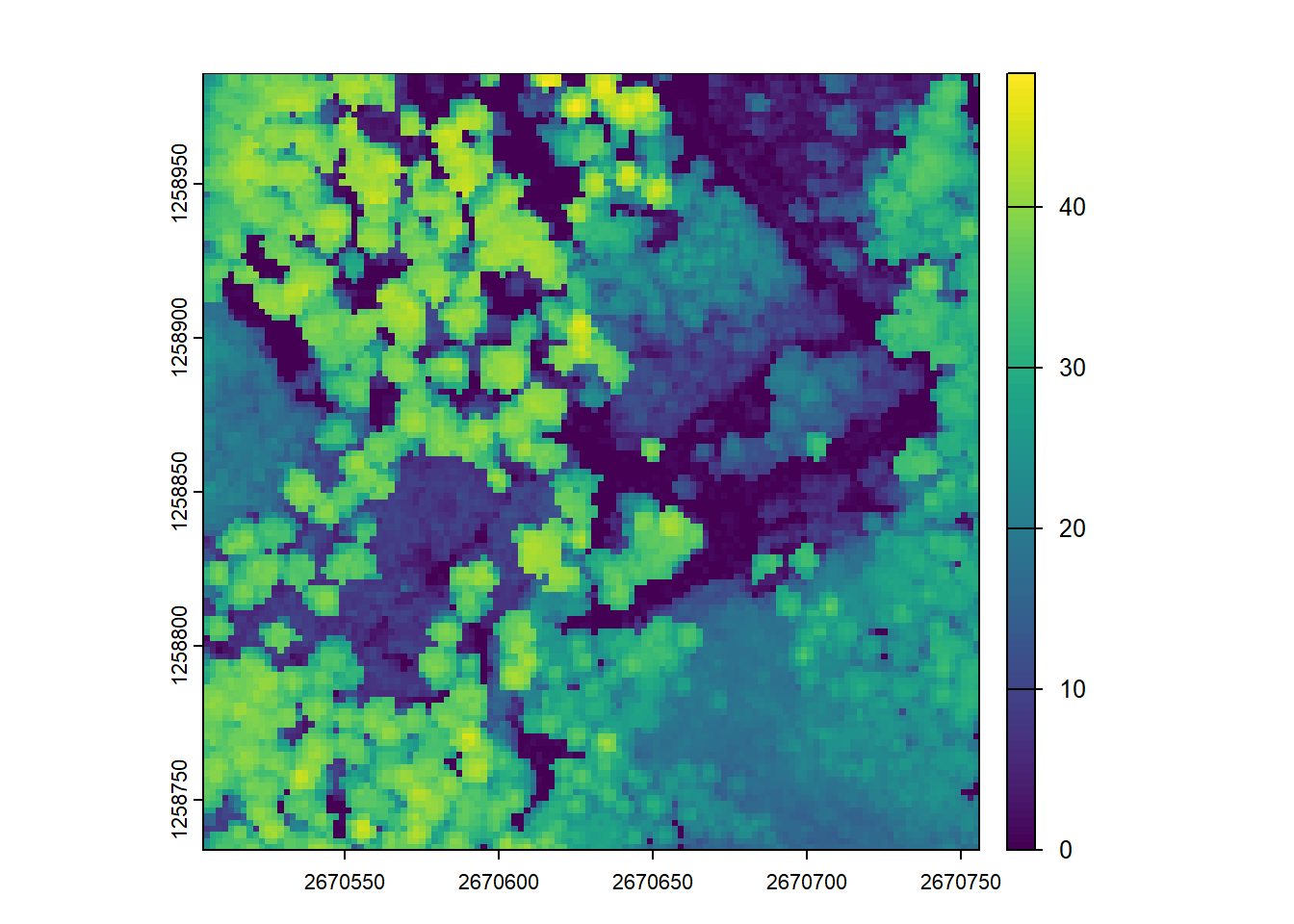

Code

plot(chm_pitfree)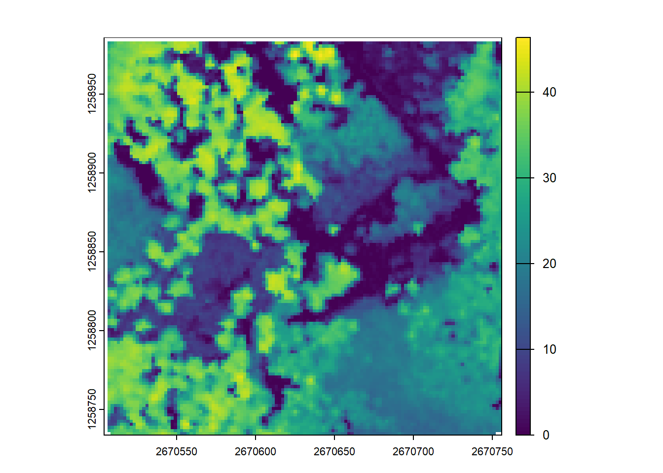

E2.

Using terra::focal() with the w = matrix(1, 5, 5) and fun = max, plot a manipulated CHM using one of the CHMs you previously generated.

Code

schm <- terra::focal(chm_pitfree, w = matrix(1, 5, ,5), fun = max, na.rm = TRUE)
plot(schm)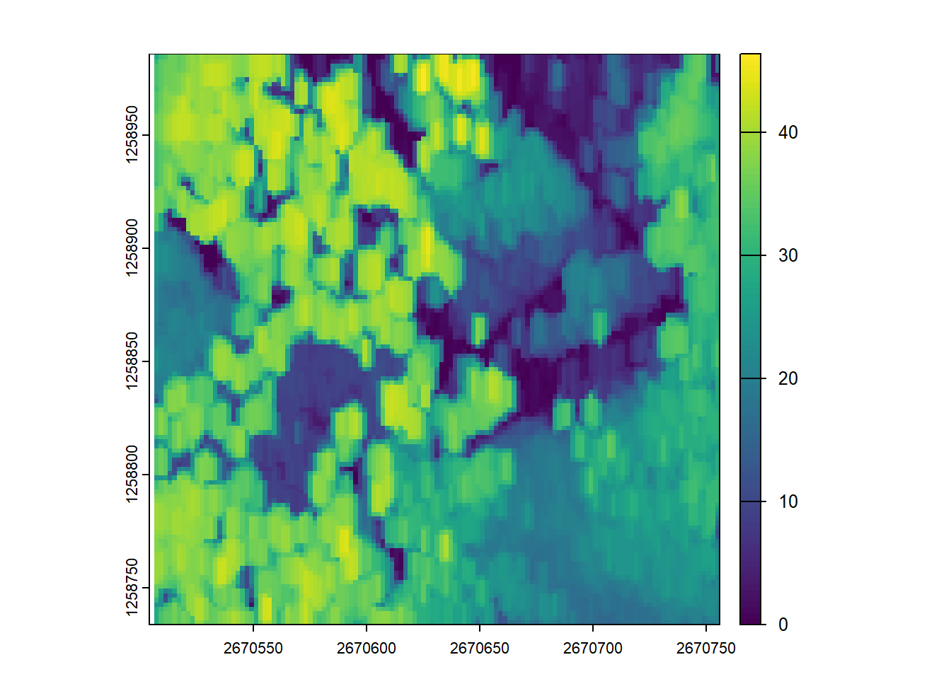

E3.

Create a 10 m CHM using a algorithm of your choice. Would this information still be useful at this scale?

Code

las <- readLAS(files = "data/zrh_norm.laz")

Code

chm <- rasterize_canopy(las=las, res=10, algorithm=p2r())
plot(chm)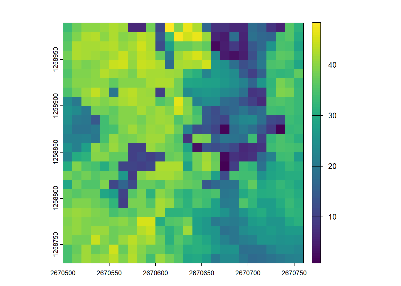

4-METRICS

E1.

Generate another metric set provided by the lidRmetrics package (voxel metrics will take too long)

Code

las <- readLAS(files = "data/zrh_norm.laz")

Code

dispersion <- pixel_metrics(las, ~metrics_percentiles(z = Z), res = 20)

E2.

Map the density of ground returns at a 5 m resolution. Hint filter = -keep_class 2

Code

las <- readLAS(files = "data/zrh_norm.laz", filter = "-keep_class 2")

Code

gnd <- pixel_metrics(las, ~length(Z)/25, res=5)
plot(gnd)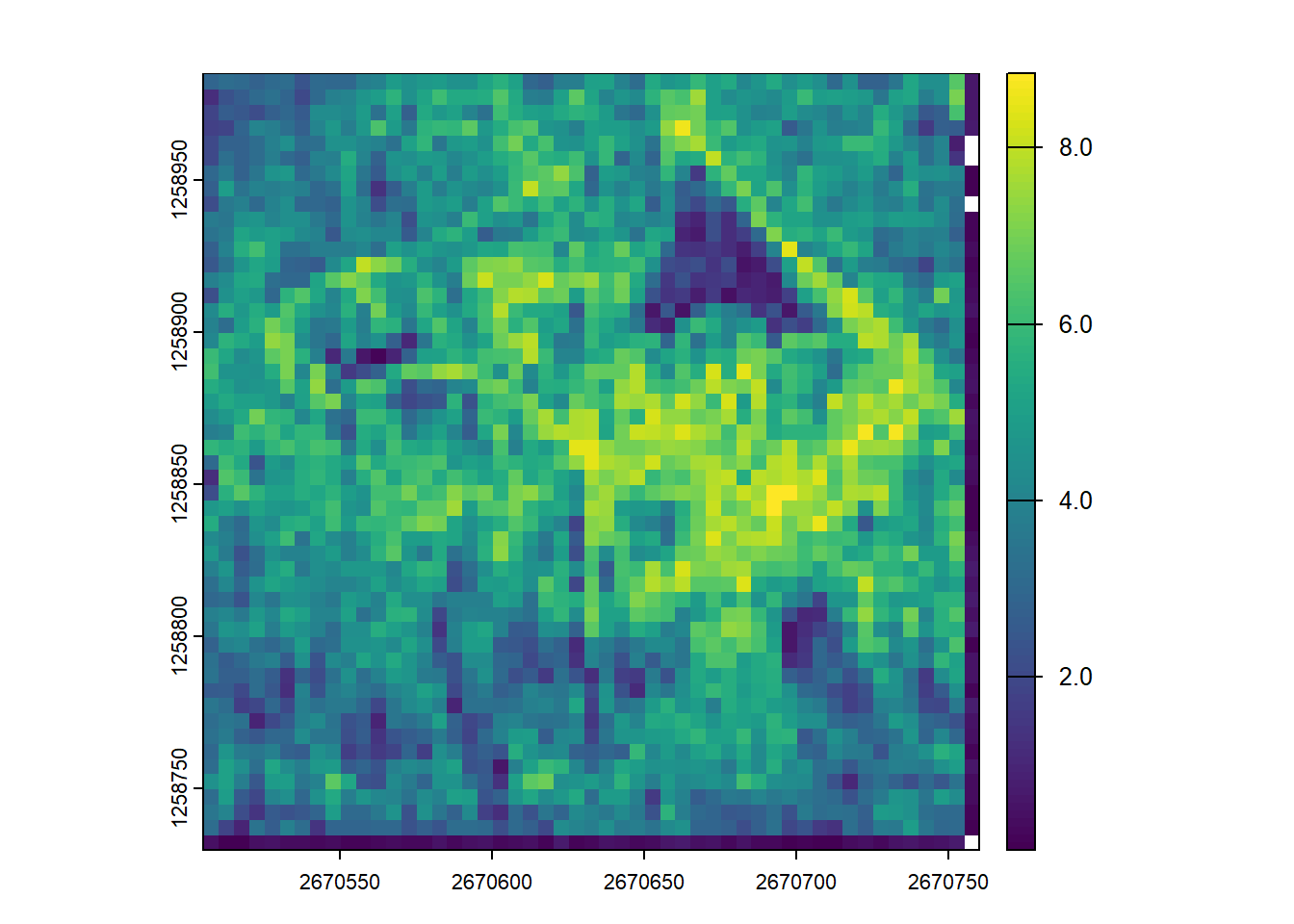

E3.

ssuming that biomass is estimated using the equation B = 0.5 * mean Z + 0.9 * 90th percentile of Z applied on first returns only, map the biomass.

Code

las <- readLAS(files = "data/zrh_norm.laz")

Code

B <- pixel_metrics(las, ~0.5*mean(Z) + 0.9*quantile(Z, probs = 0.9), 10, filter = ~ReturnNumber == 1L)
plot(B)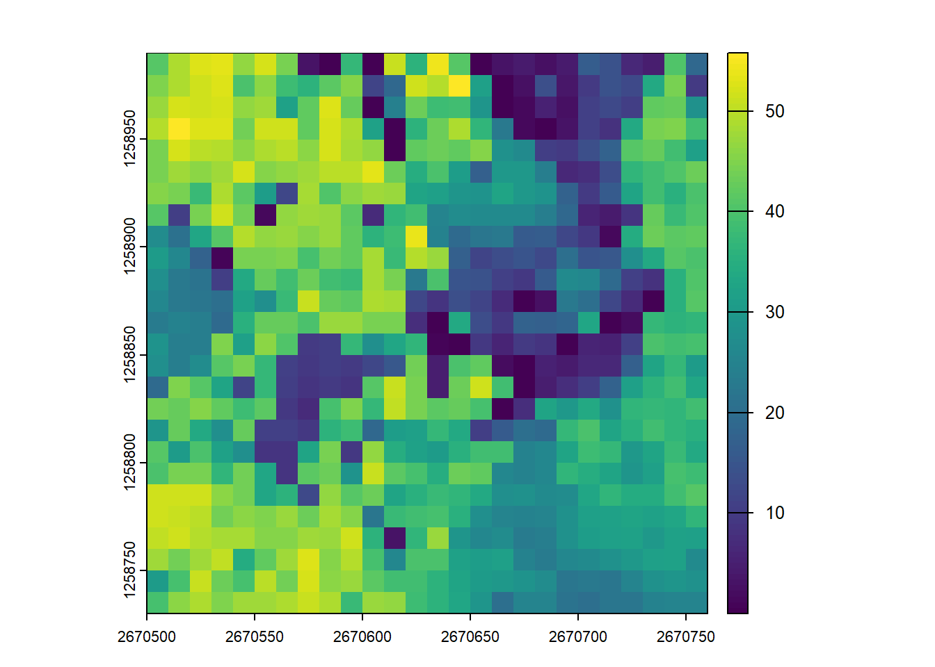

6-LASCATALOG

E1.

Calculate a set of metrics from the lidRmetrics package on the catalogue (voxel metrics will take too long)

Code

ctg <- readLAScatalog(folder = "data/ctg_norm")
dispersion <- pixel_metrics(ctg, ~metrics_dispersion(z = Z, dz = 2, zmax = 30), res = 20)

#> Chunk 1 of 9 (11.1%): state ✓
#> 
                                                                                
Chunk 2 of 9 (22.2%): state ✓
#> 
                                                                                
Chunk 3 of 9 (33.3%): state ✓
#> 
                                                                                
Chunk 4 of 9 (44.4%): state ✓
#> 
                                                                                
Chunk 5 of 9 (55.6%): state ✓
#> 
                                                                                
Chunk 6 of 9 (66.7%): state ✓
#> 
                                                                                
Chunk 7 of 9 (77.8%): state ✓
#> 
                                                                                
Chunk 8 of 9 (88.9%): state ✓
#> 
                                                                                
Chunk 9 of 9 (100%): state ✓
#> 
                                                                                
plot(dispersion)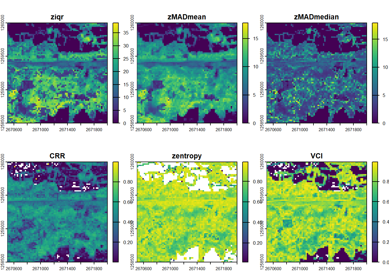

E2.

Read in the non-normalized las catalog filtering the point cloud to only include first returns.

Code

ctg <- readLAScatalog(folder = "data/ctg_class")
opt_filter(ctg) <- "-keep_first -keep_class 2"

E3.

Generate a DTM at 1m spatial resolution for the provided catalog with only first returns.

Code

dtm_first <- rasterize_terrain(ctg, res = 1, algorithm = tin())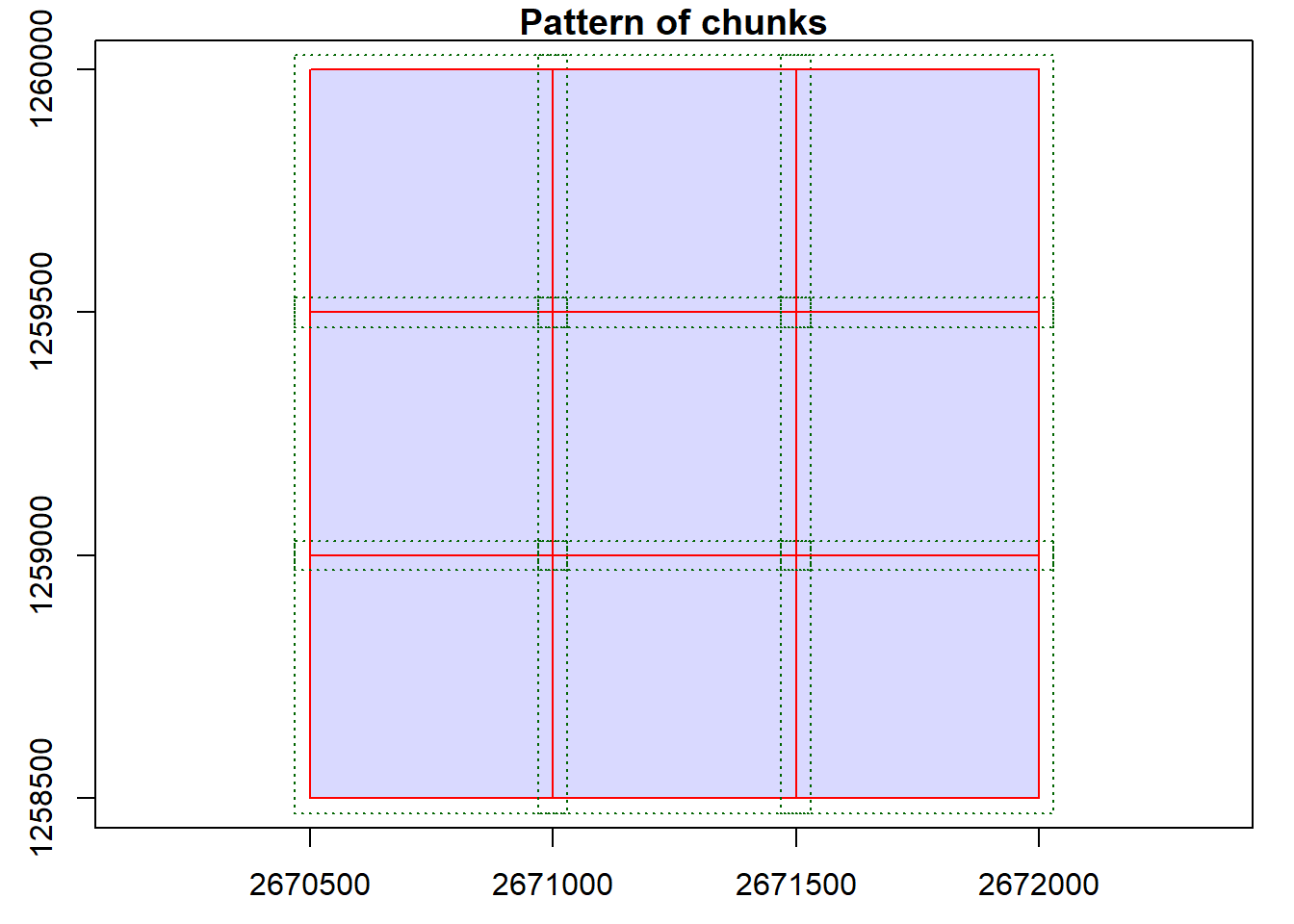

#> Chunk 1 of 9 (11.1%): state ✓
#> 
                                                                                
Chunk 2 of 9 (22.2%): state ✓
#> 
                                                                                
Chunk 3 of 9 (33.3%): state ✓
#> 
                                                                                
Chunk 4 of 9 (44.4%): state ✓
#> 
                                                                                
Chunk 5 of 9 (55.6%): state ✓
#> 
                                                                                
Chunk 6 of 9 (66.7%): state ✓
#> 
                                                                                
Chunk 7 of 9 (77.8%): state ✓
#> 
                                                                                
Chunk 8 of 9 (88.9%): state ✓
#> 
                                                                                
Chunk 9 of 9 (100%): state ✓
#> 
                                                                                
plot(dtm_first)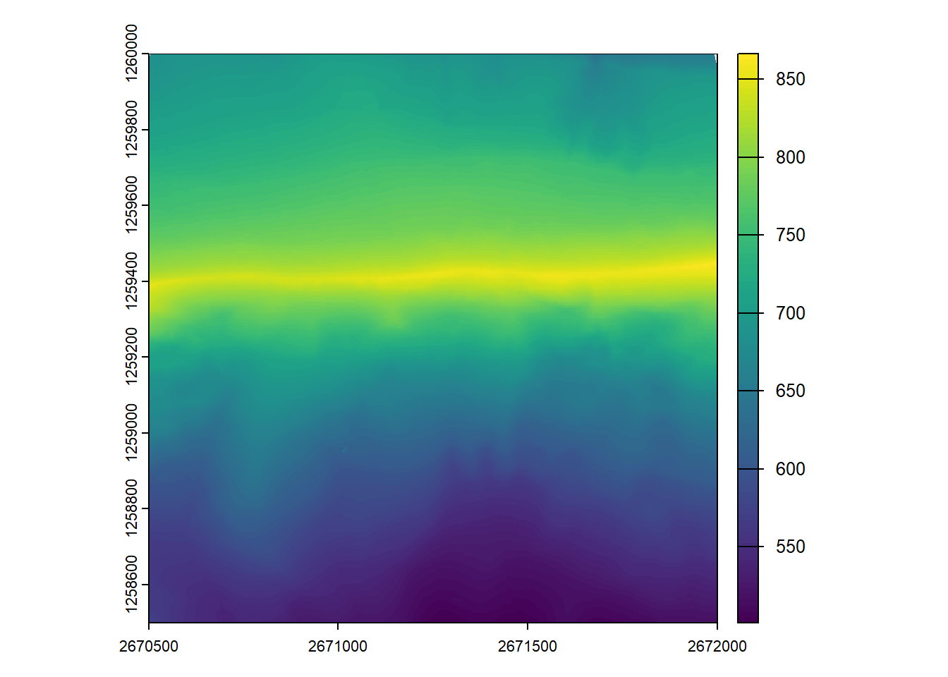

Tip

The Multiple Returns and Canopy Penetration This exercise highlights a critical and unique capability of Airborne Laser Scanning (ALS).

Unlike methods based on imagery like Digital Aerial Photogrammetry (DAP), map the visible surface, LiDAR pulses can penetrate through gaps in the vegetation generating multiple returns each. This allows us to map the ground surface even under dense forest cover, which is essential for creating accurate Digital Terrain Models (DTMs).