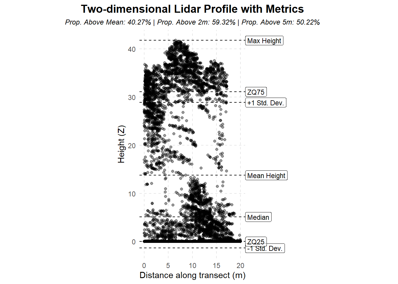
zrh_norm.laz some metrics are generated and presented alongside the coordinates of the points within this example cellThis code demonstrates an example of generating pixel-based summary metrics of lidar data. This is a common task to capture critical information describing the vertical distribution of lidar returns across a regular grid (raster). Pixel metrics are used in various predictive modelling tasks and often to capture critical vegetation characteristics ranging from height to variability and cover.
Beyond statistical summary metrics such as (mean, max, sd, etc), many researchers have developed custom metrics linked to critical vegetation attributes such as leaf-area index, vertical complexity indices, etc.
Additional metrics can also be generated with lidR using voxel approaches, where three-dimensional sub-compartments are fit to better capture complexity — at the cost of vastly increasing computational requirements and introducing additional parameters.
Classically, lidar metrics used in vegetation characterization typically fall under three categories:
Height metrics
These typically describe how tall the vegetation generally is. Often max height, mean height, and percentiles of height are important in the prediction of attributes including land cover, and continuous variables like biomass.
Variability metrics
Metrics describing the shape of the distribution of returns often capture additional signals useful for explaining the level of vegetation complexity within a pixel. Skewed versus bimodal distributions, for example, can represent a very dense upper canopy in a forest compared to a multi-layer stand.
Cover metrics
Often referred directly to as canopy cover, these metrics generally describe the proportion of returns (as a %) above a certain threshold. Typically used to generally describe how much vegetation (e.g. above 2m) there is compared to ground and other lower surfaces (designed for forest).
zrh_norm.laz some metrics are generated and presented alongside the coordinates of the points within this example cell# Clear environment
rm(list = ls(globalenv()))
# Load packages
library(lidR)
library(terra)
library(lidRmetrics)To begin we compute simple metrics including mean and max height of points within 10x10 m pixels and visualizing the results. The code shows how to compute multiple metrics simultaneously and use predefined metric sets. Advanced usage introduces user-defined metrics for more specialized calculations.
# Load the normalized lidar data
las <- readLAS(files = "data/zrh_norm.laz")
The pixel_metrics() function calculates structural metrics within a defined spatial resolution (res).
# Compute the mean height of points within 10x10 m pixels
hmean <- pixel_metrics(las = las, func = ~mean(Z), res = 10)
hmean
#> class       : SpatRaster
#> dimensions  : 26, 26, 1  (nrow, ncol, nlyr)
#> resolution  : 10, 10  (x, y)
#> extent      : 2670500, 2670760, 1258730, 1258990  (xmin, xmax, ymin, ymax)
#> coord. ref. : CH1903+ / LV95 (EPSG:2056)
#> source(s)   : memory
#> name        :          V1
#> min value   :  0.01491925
#> max value   : 28.90163739
plot(hmean)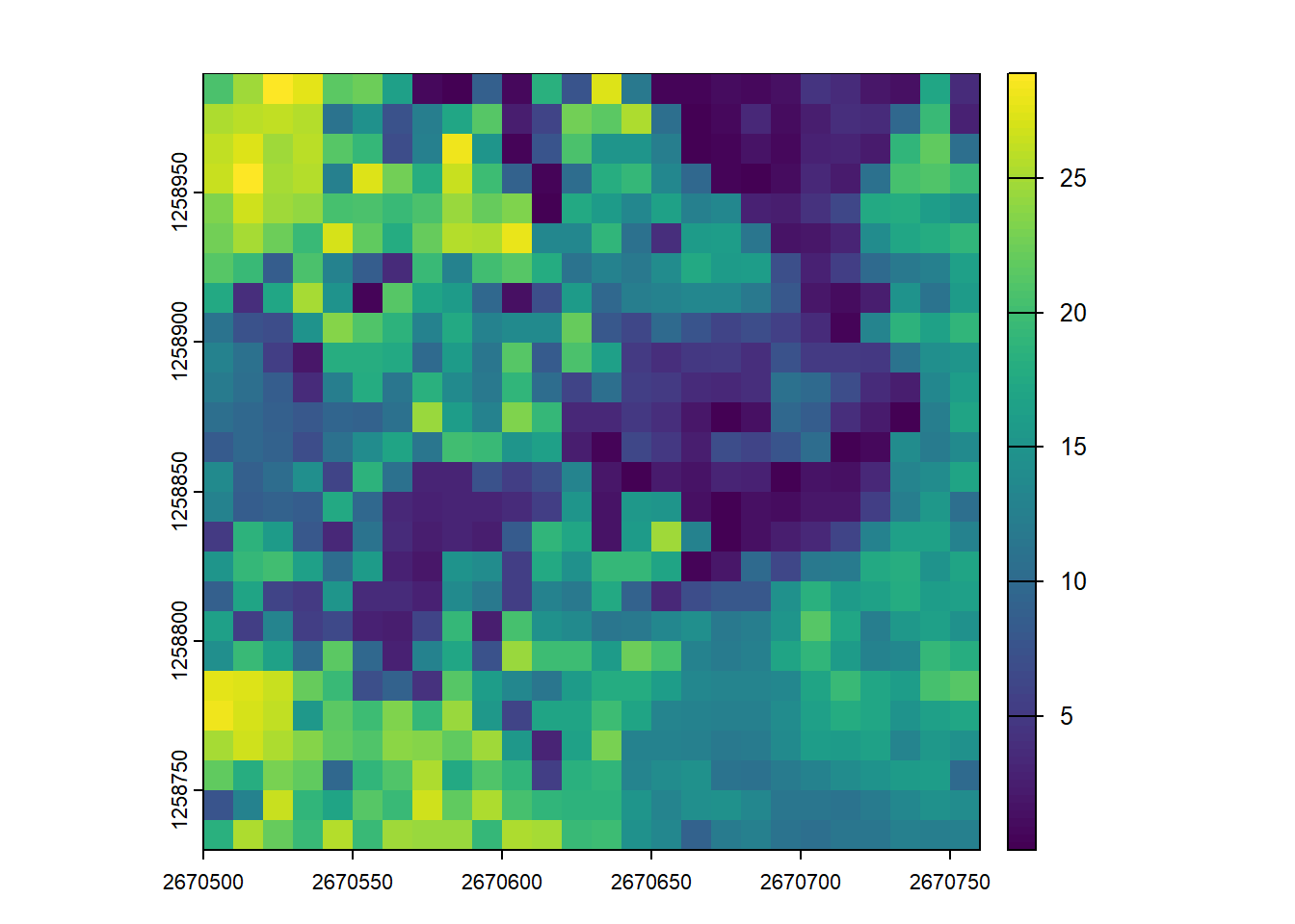
# Compute the max height of points within 10x10 m pixels
hmax <- pixel_metrics(las = las, func = ~max(Z), res = 10)
hmax
#> class       : SpatRaster
#> dimensions  : 26, 26, 1  (nrow, ncol, nlyr)
#> resolution  : 10, 10  (x, y)
#> extent      : 2670500, 2670760, 1258730, 1258990  (xmin, xmax, ymin, ymax)
#> coord. ref. : CH1903+ / LV95 (EPSG:2056)
#> source(s)   : memory
#> name        :    V1
#> min value   :  0.93
#> max value   : 48.31
plot(hmax)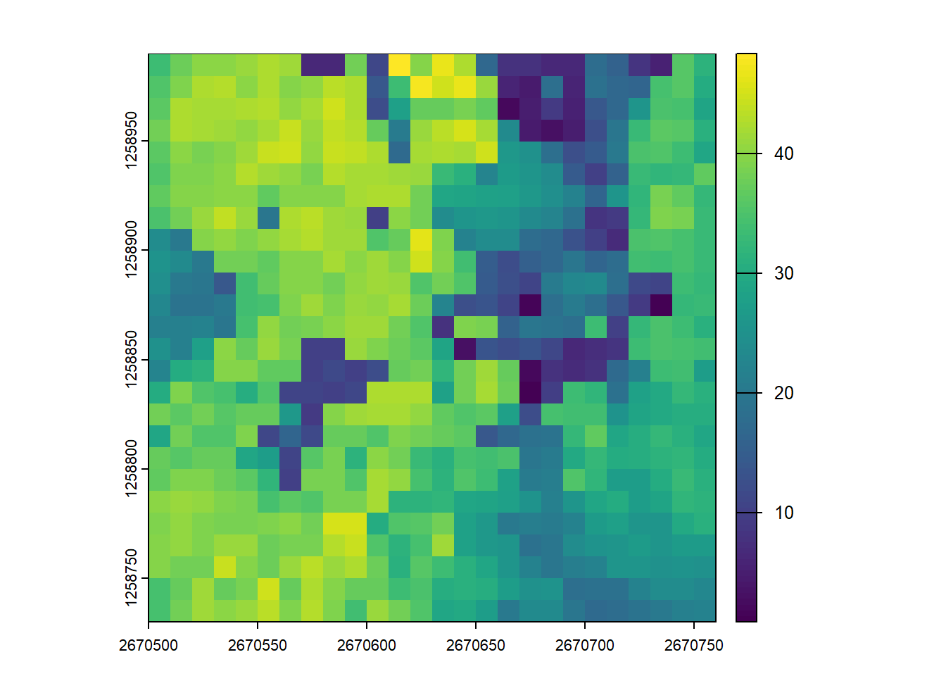
You can specify that multiple metrics should be calculated by housing them in a list().
# Compute several metrics at once using a list
metrics <- pixel_metrics(las = las, func = ~list(hmax = max(Z), hmean = mean(Z)), res = 10)
metrics
#> class       : SpatRaster
#> dimensions  : 26, 26, 2  (nrow, ncol, nlyr)
#> resolution  : 10, 10  (x, y)
#> extent      : 2670500, 2670760, 1258730, 1258990  (xmin, xmax, ymin, ymax)
#> coord. ref. : CH1903+ / LV95 (EPSG:2056)
#> source(s)   : memory
#> names       :  hmax,       hmean
#> min values  :  0.93,  0.01491925
#> max values  : 48.31, 28.90163739
plot(metrics)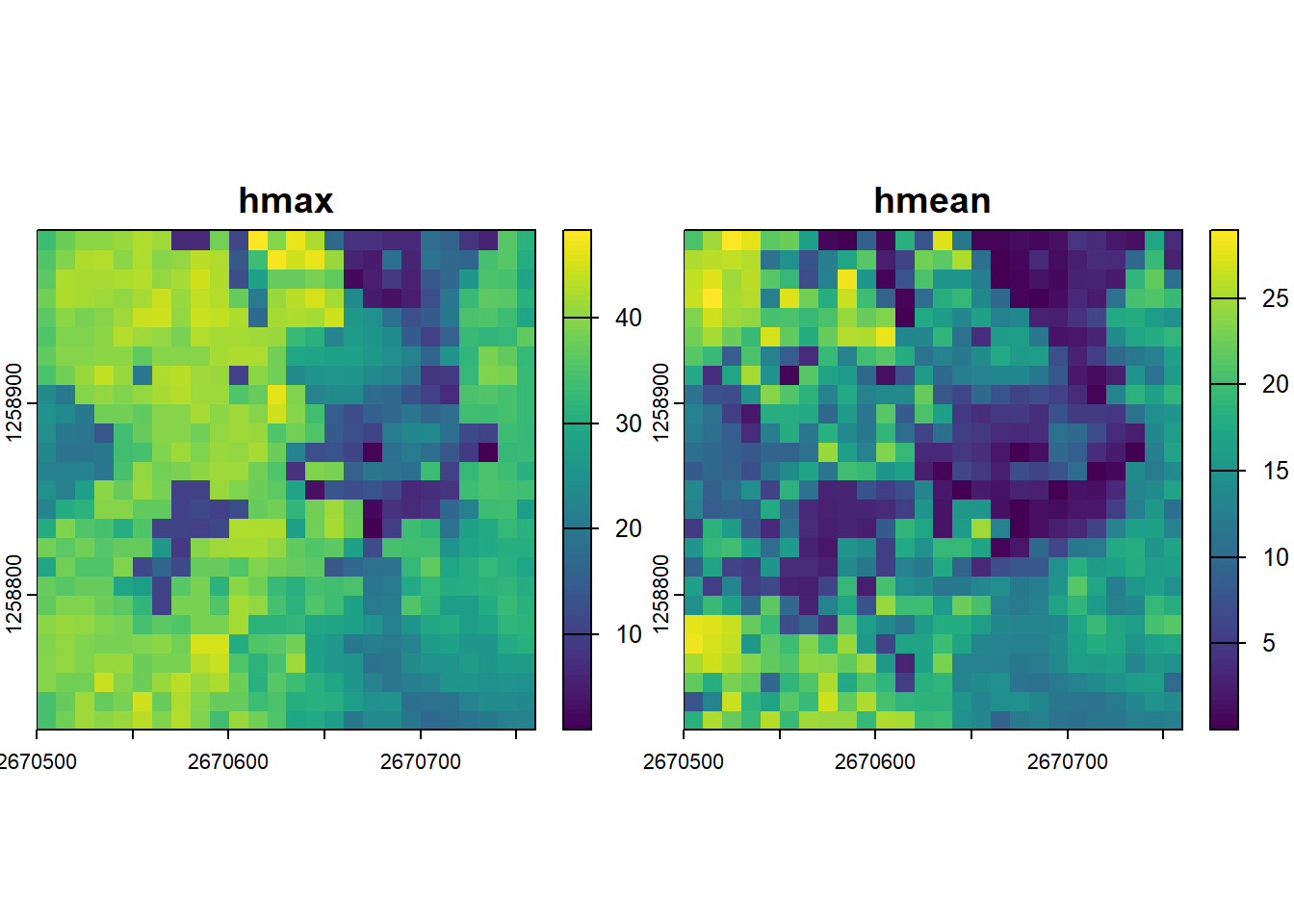
Pre-defined metric sets are available, such as .stdmetrics_z. See more here.
# Simplify computing metrics with predefined sets of metrics
metrics <- pixel_metrics(las = las, func = .stdmetrics_z, res = 10)
metrics
#> class       : SpatRaster
#> dimensions  : 26, 26, 36  (nrow, ncol, nlyr)
#> resolution  : 10, 10  (x, y)
#> extent      : 2670500, 2670760, 1258730, 1258990  (xmin, xmax, ymin, ymax)
#> coord. ref. : CH1903+ / LV95 (EPSG:2056)
#> source(s)   : memory
#> names       :  zmax,       zmean,         zsd,     zskew,      zkurt,   zentropy, ...
#> min values  :  0.93,  0.01491925,  0.07074514, -2.027288,   1.109003, 0.02902023, ...
#> max values  : 48.31, 28.90163739, 17.97744082, 16.645088, 308.212065, 0.93158775, ...
plot(metrics)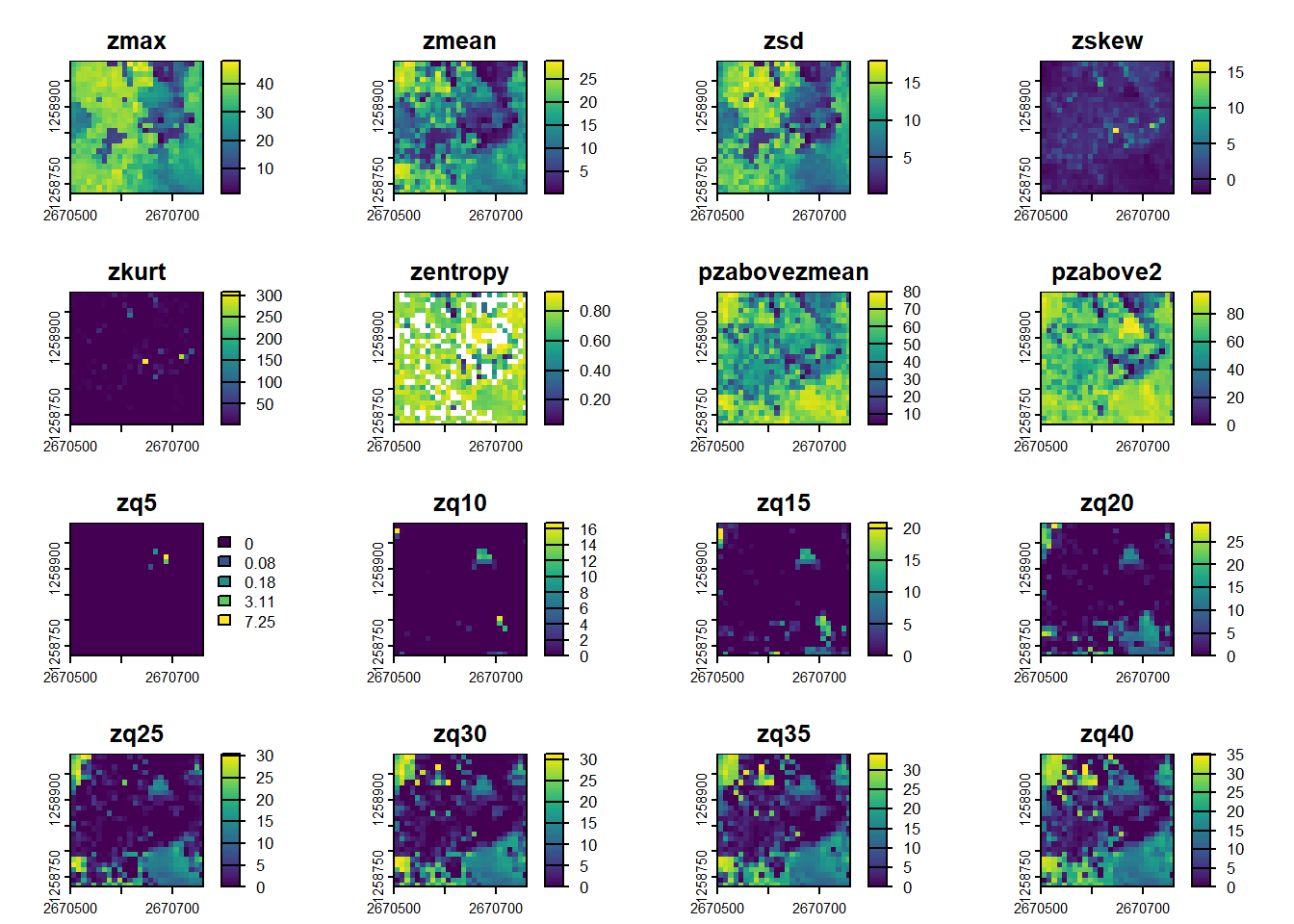
.stdmetrics_z set.
We can examine the distribution of the standard deviation of return heights across the 10m grid cells by sub-setting this metric and plotting the raster. Even this simple metric demonstrates the variability in vertical vegetation structure across this dataset.
# Plot a specific metric from the predefined set
plot(metrics, "zsd")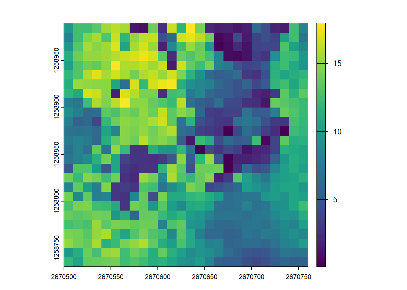
zsd), a metric from the .stdmetrics_z set.
lidR provides flexibility for users to define custom metrics. Check out 3rd party packages like lidRmetrics for suites of advanced metrics typically demonstrated in peer-reviewed articles and implemented in lidR through lidRmetrics.
We will present several metrics often tied to vegetation and biodiversity, for an overview of connecting metrics with habitat see this article.
Canopy cover is often estimated using the proportion of lidar returns generated over some threshold. Two metres is commonly used, ultimately canopy cover seeks to quantify relatively how much vegetation (points) is present.
cc_metrics <- pixel_metrics(las, func = ~metrics_percabove(z = Z, threshold = 2, zmin = 0), res = 10)
plot(cc_metrics)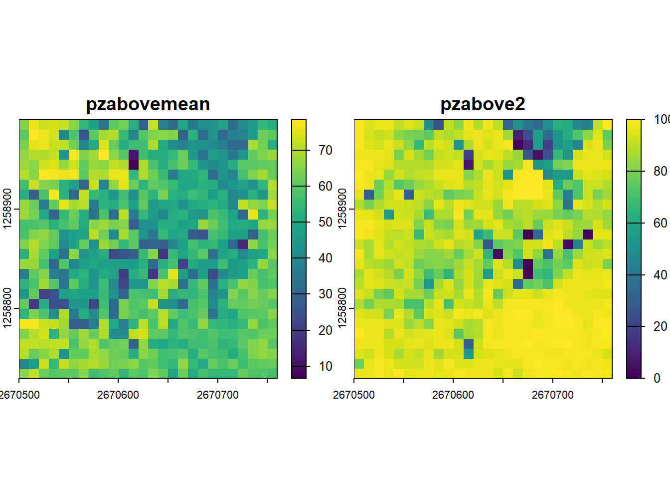
Leaf Area Density Profiles (Bouvier et al. 2015)
Leaf Area Density (LAD) profiles describe the vertical distribution of foliage within the canopy. The method estimates the amount of leaf material in successive horizontal layers by modeling how lidar pulses are intercepted as they travel down through the vegetation.
lad_metrics <- pixel_metrics(las, ~metrics_lad(z = Z), res = 10)
plot(lad_metrics)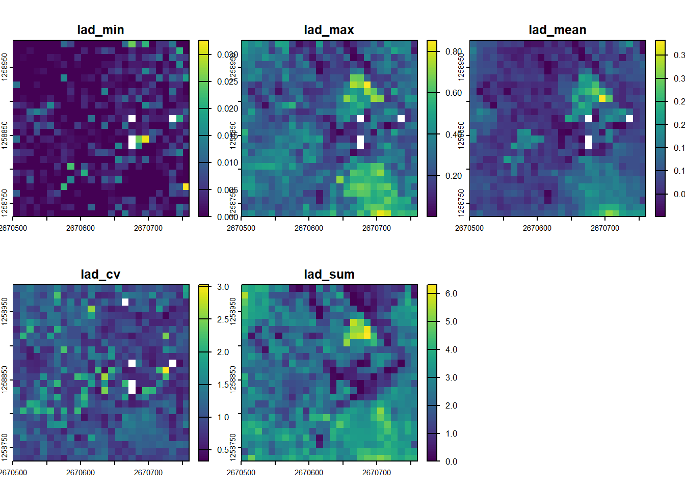
The Coefficient of Variation of LAD (lad_cv) quantifies the uniformity of the vertical foliage distribution. A high lad_cv value indicates that foliage is concentrated in a specific layer (e.g., a simple, even-aged canopy), while a low value suggests foliage is more evenly spread across multiple layers, indicating greater vertical complexity.
plot(lad_metrics, "lad_cv")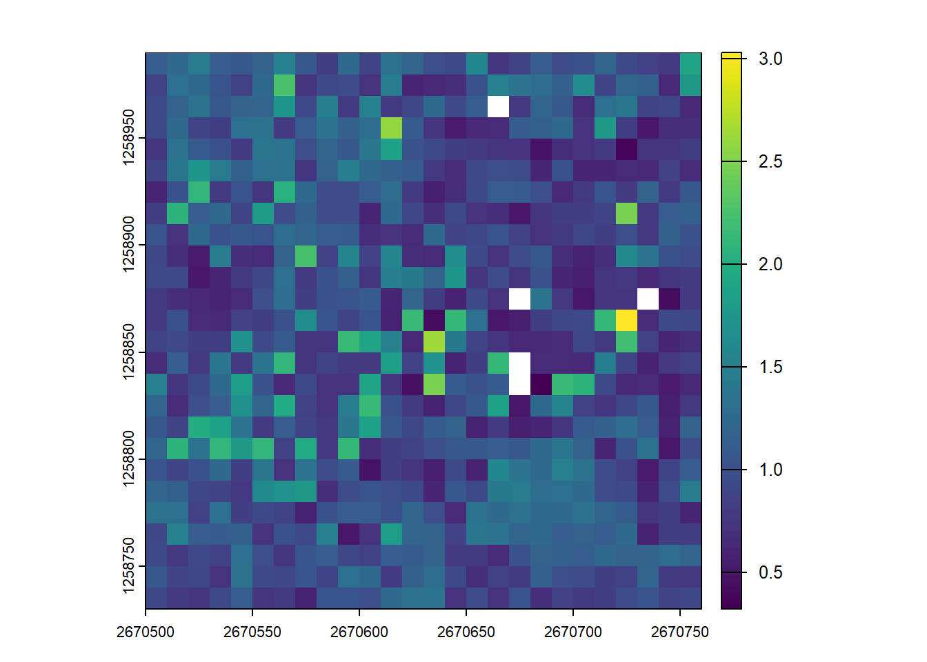
Dispersion and Vertical Complexity
While standard deviation (zsd) gives a general sense of height variability, dispersion metrics provide a more nuanced characterization of how lidar points are distributed vertically within the canopy. They help quantify the structural complexity of vegetation, which is crucial for applications like habitat modeling and biomass estimation.
# Calculate several dispersion metrics. zmax is required to compute VCI.
disp_metrics <- pixel_metrics(las, ~metrics_dispersion(z = Z, zmax = 40), res = 10)
plot(disp_metrics)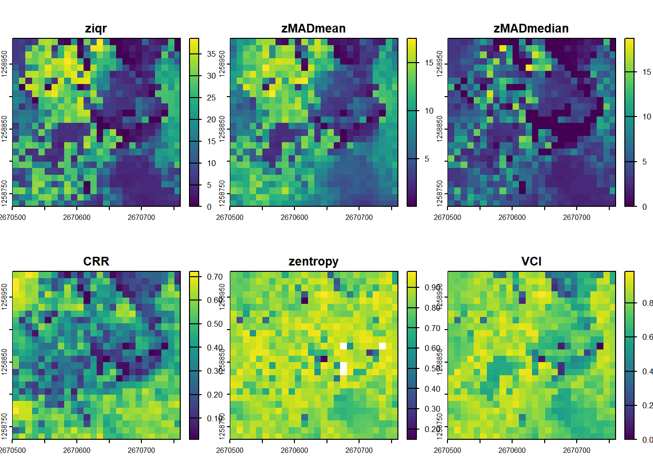
Canopy Relief Ratio (CRR) measures the position of the mean point height relative to the overall height range of the canopy. It is calculated as (mean(Z) - min(Z)) / (max(Z) - min(Z)). A value closer to 1 suggests that most of the vegetation volume is concentrated in the upper parts of the canopy.
plot(disp_metrics, "CRR")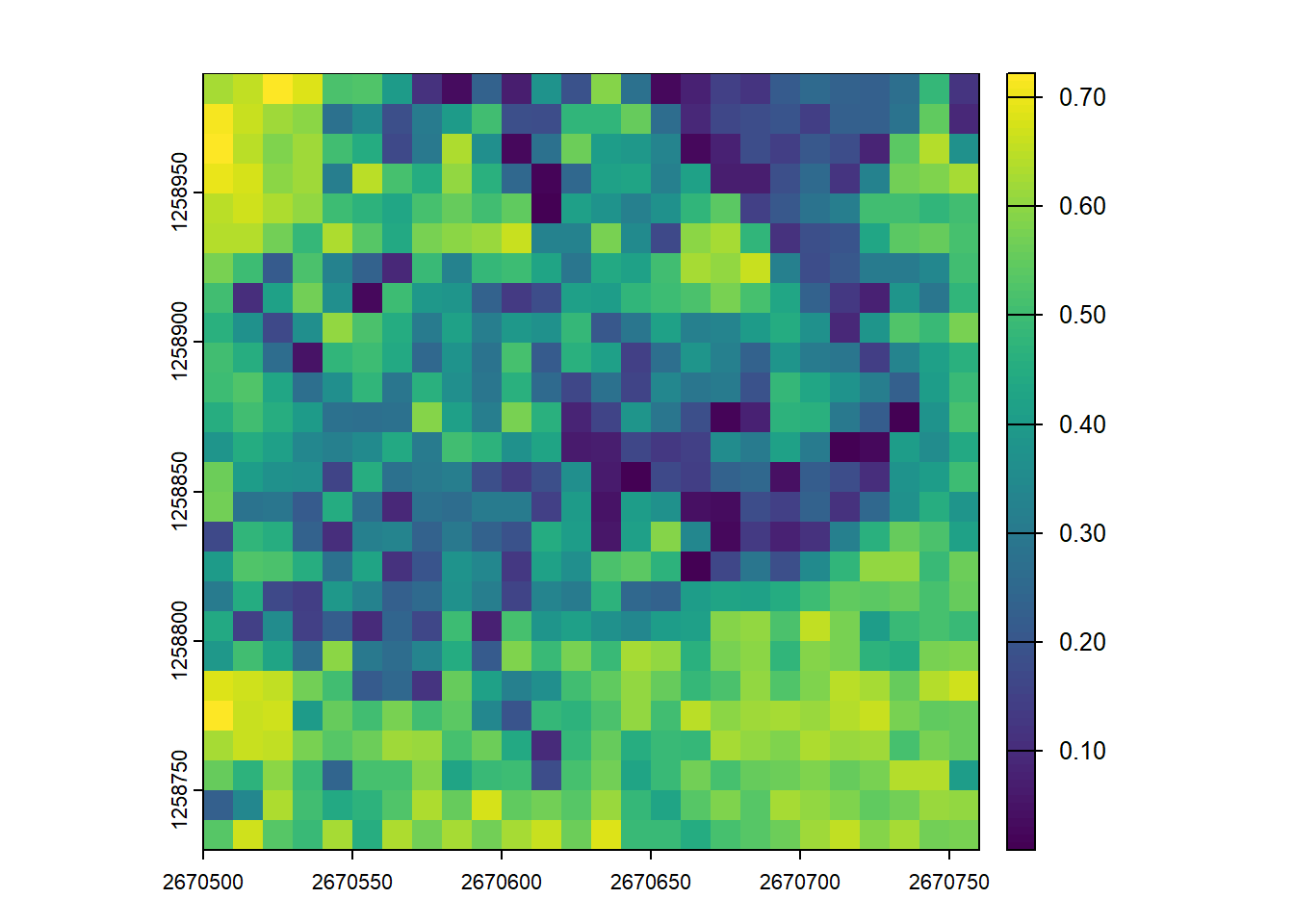
Vertical Complexity Index (VCI) uses entropy to quantify how evenly the lidar returns are distributed throughout the vertical profile. Higher VCI values indicate a more complex, multi-layered canopy structure (e.g., a forest with understory, mid-story, and overstory). Lower values suggest a simpler structure where points are clumped at specific heights (e.g., a field of grass or a dense, flat-topped plantation).
plot(disp_metrics, "VCI")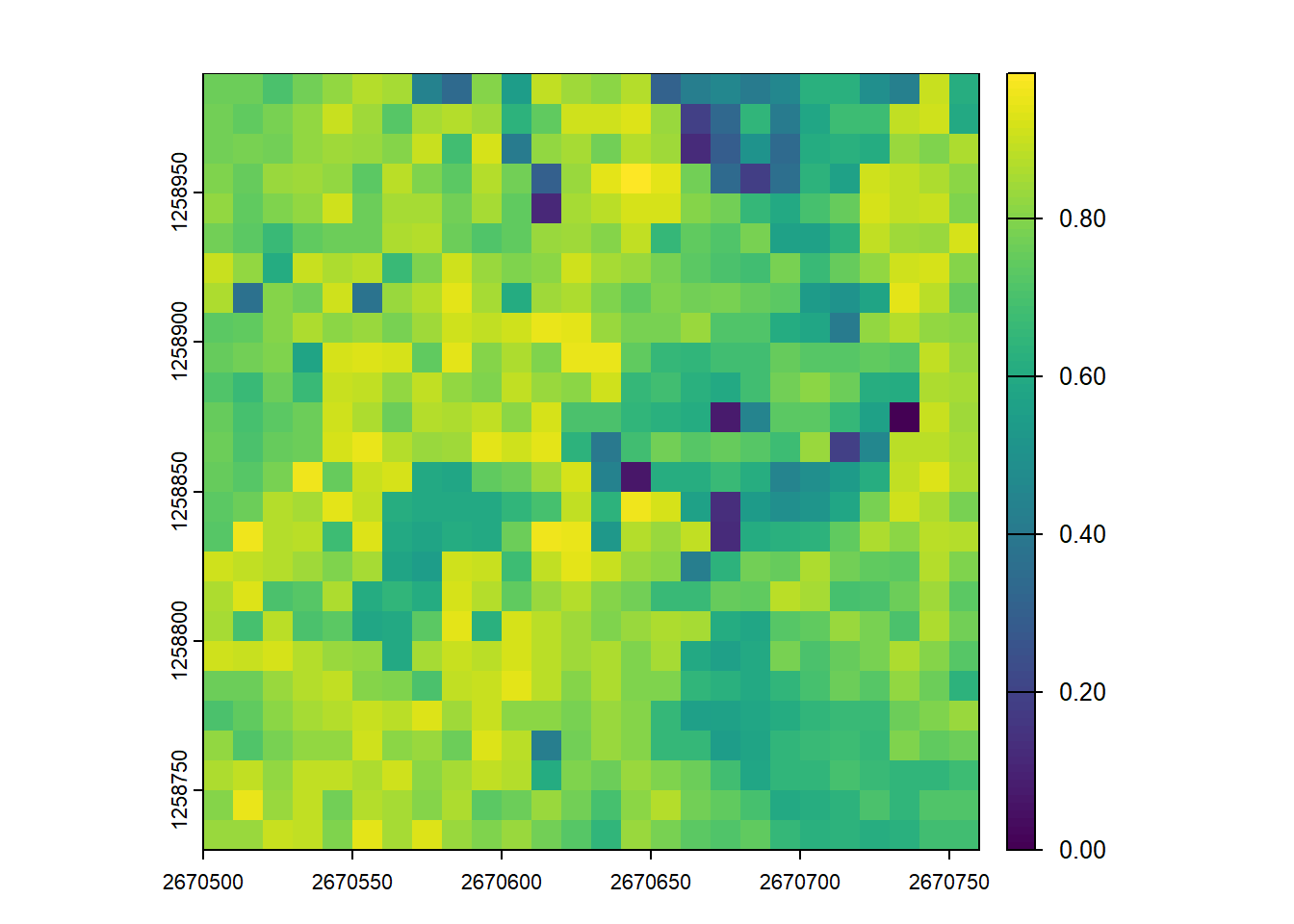
User Defined Metrics
We can also create our own user-defined metric functions. This demonstrates the flexibility of the lidR package!
Here we generate an arbitrary function to compute a weighted mean between two attributes. We then calculate the mean height of 10 m pixels weighted by return Intensity (albeit a potentially meaningless metric)
# Generate a user-defined function to compute weighted mean between two attributes
f <- function(x, weight) { sum(x*weight)/sum(weight) }

# Compute weighted mean of height (Z) as a function of return intensity
user_metric <- pixel_metrics(las = las, func = ~f(Z, Intensity), res = 10)

# Visualize the output
plot(user_metric)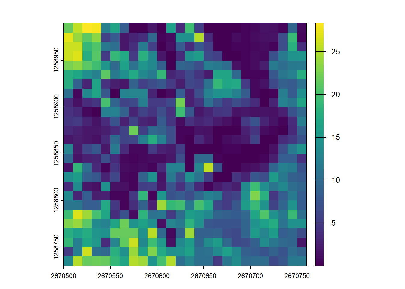
Using:
las <- readLAS("data/zrh_norm.laz")Generate another metric set provided by the lidRmetrics package (voxel metrics will take too long)
Map the density of ground returns at a 5 m resolution (in points/m2). Hints: filter = -keep_class 2 - what’s the area of a 5 m pixel?
Assuming that biomass is estimated using the equation B = 0.5 * mean Z + 0.9 * 90th percentile of Z applied on first returns only, map the biomass.
In this tutorial, we covered basic usage of the lidR package for computing mean and max heights within grid cells and using predefined sets of metrics. Additionally, we explored the advanced usage with the ability to define user-specific metrics for grid computation.