Excercise Solutions

Resources

Code

1-LAS

# Load packages
library(sf)
library(terra)
library(lidR)
library(lidRmetrics)

E1.

Using the plot() function plot the point cloud with a different attribute that has not been done yet

Try adding axis = TRUE, legend = TRUE to your plot argument plot(las, axis = TRUE, legend = TRUE)

Code

las <- readLAS(files = "data/fm_norm.laz")

Code

plot(las, color = "ReturnNumber", axis = TRUE, legend = TRUE)

E2.

Create a filtered las object of returns that have an Intensity greater that 50, and plot it.

Code

las <- readLAS(files = "data/fm_norm.laz")

Code

i_50 <- filter_poi(las = las, Intensity > 50)
plot(i_50)

E3.

Read in the las file with only xyz and intensity only. Hint go to the lidRbook section to find out how to do this.

Code

las <- readLAS(files = "data/fm_norm.laz", select = "xyzi")

2-DTM

E1.

Compute two DTMs for this point cloud with differing spatial resolutions, plot both e.g. `plot(dtm1)

Code

las <- readLAS(files = "data/fm_class.laz")

Code

dtm_5 <- rasterize_terrain(las=las, res=5, algorithm=tin())
dtm_10 <- rasterize_terrain(las=las, res=10, algorithm=tin())
plot(dtm_5)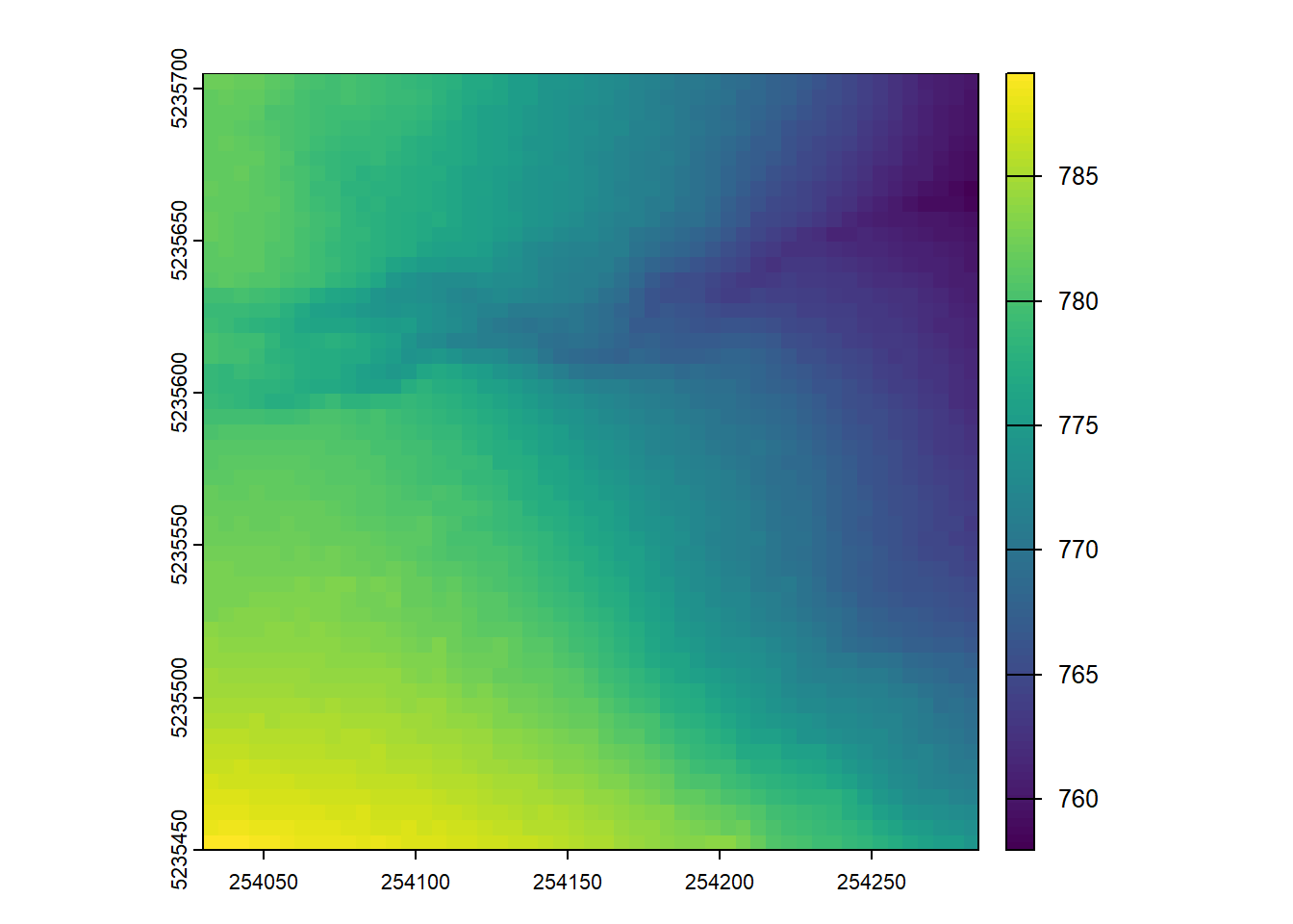

Code

plot(dtm_10)

E2.

Now use the plot_dtm3d() function to visualize and move around your newly created DTMs

Code

plot_dtm3d(dtm_5)

3-CHM

E1.

Using the p2r() and pitfree() (defining your own arguments) create two CHMs with the same resolution and plot them. What differences do you notice?

Code

las <- readLAS(files = "data/fm_norm.laz")

Code

chm_p2r <- rasterize_canopy(las=las, res=2, algorithm=p2r())

thresholds <- c(0, 5, 10, 20, 25, 30)
max_edge <- c(0, 1.35)
chm_pitfree <- rasterize_canopy(las = las, res = 2, algorithm = pitfree(thresholds, max_edge))

plot(chm_p2r)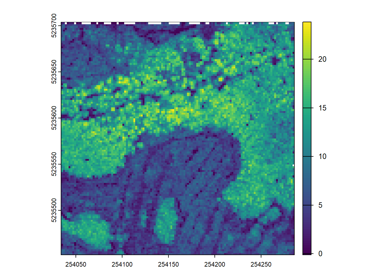

Code

plot(chm_pitfree)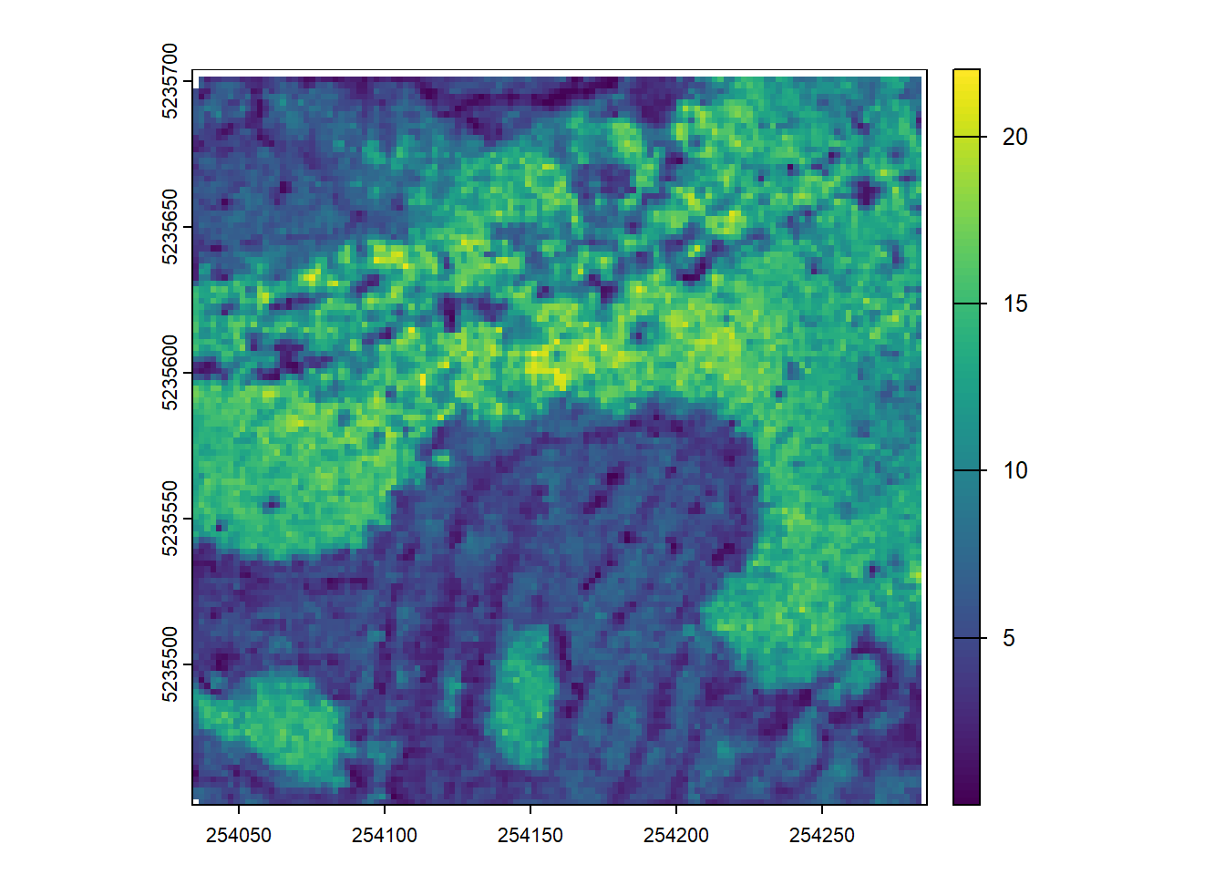

E2.

Using terra::focal() with the w = matrix(1, 5, 5) and fun = max, plot a manipulated CHM using one of the CHMs you previously generated.

Code

schm <- terra::focal(chm_pitfree, w = matrix(1, 5, ,5), fun = max, na.rm = TRUE)
plot(schm)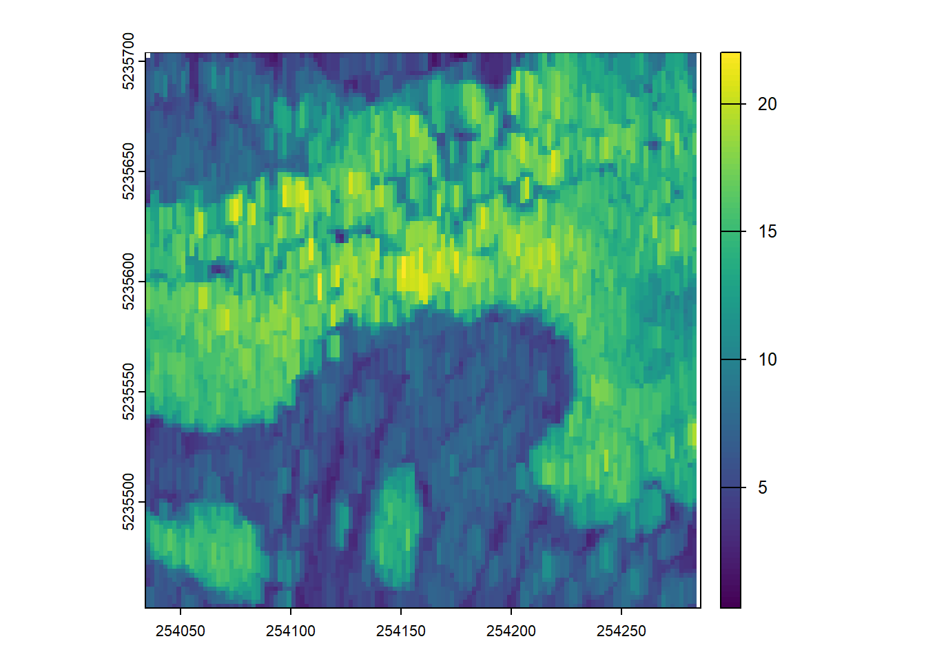

E3.

Create a 10 m CHM using a algorithm of your choice. Would this information still be useful at this scale?

Code

las <- readLAS(files = "data/fm_norm.laz")

Code

chm <- rasterize_canopy(las=las, res=10, algorithm=p2r())
plot(chm)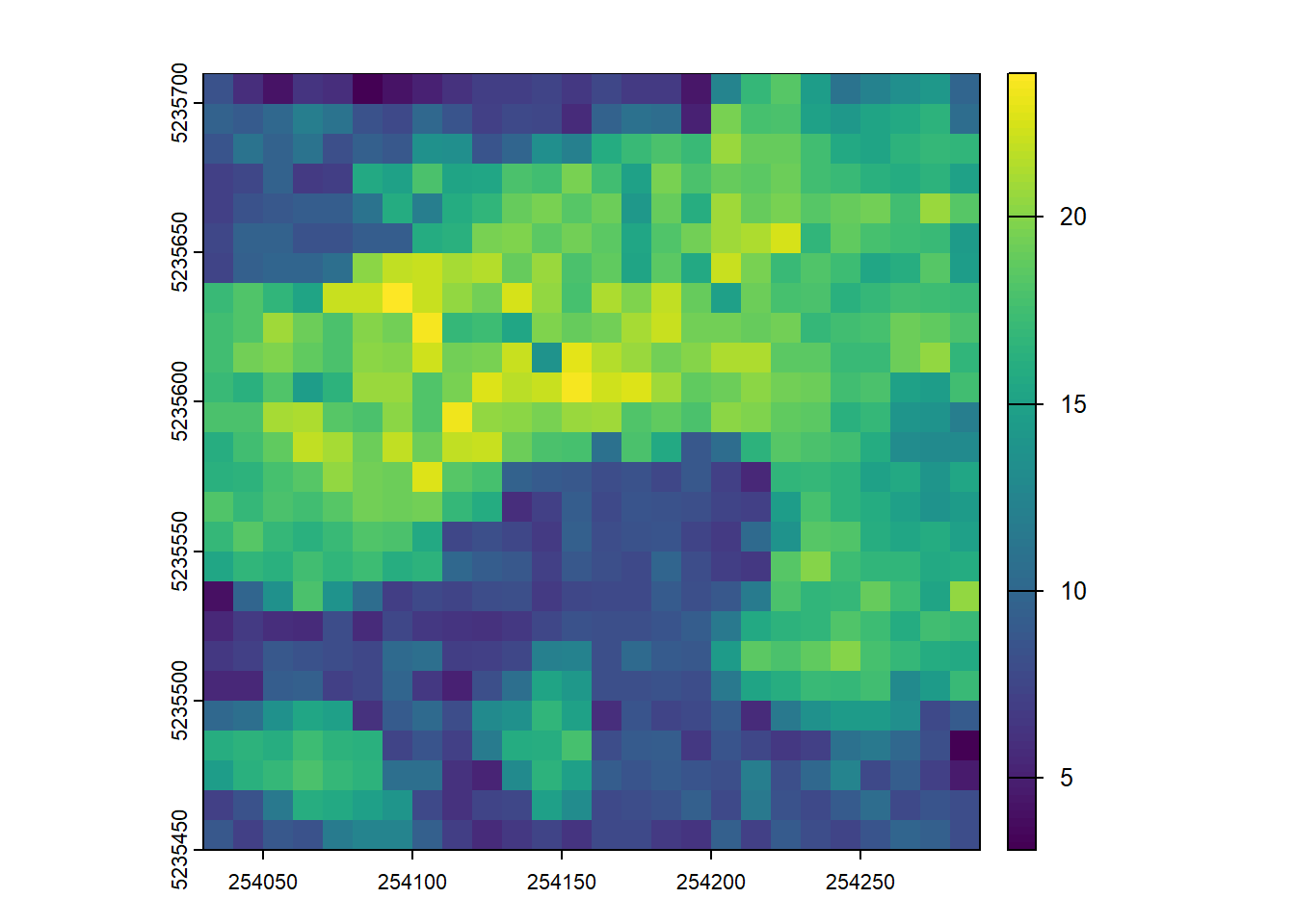

4-METRICS

E1.

Generate another metric set provided by the lidRmetrics package (voxel metrics will take too long)

Code

las <- readLAS(files = "data/fm_norm.laz")

Code

dispersion <- pixel_metrics(las, ~metrics_percentiles(z = Z), res = 20)

E2.

Map the density of ground returns at a 5 m resolution. Hint filter = -keep_class 2

Code

las <- readLAS(files = "data/fm_norm.laz", filter = "-keep_class 2")

Code

gnd <- pixel_metrics(las, ~length(Z)/25, res=5)
plot(gnd)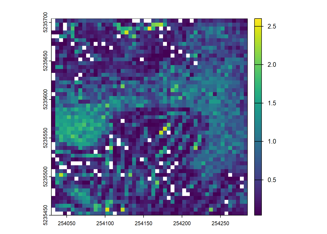

E3.

ssuming that biomass is estimated using the equation B = 0.5 * mean Z + 0.9 * 90th percentile of Z applied on first returns only, map the biomass.

Code

las <- readLAS(files = "data/fm_norm.laz")

Code

B <- pixel_metrics(las, ~0.5*mean(Z) + 0.9*quantile(Z, probs = 0.9), 10, filter = ~ReturnNumber == 1L)
plot(B)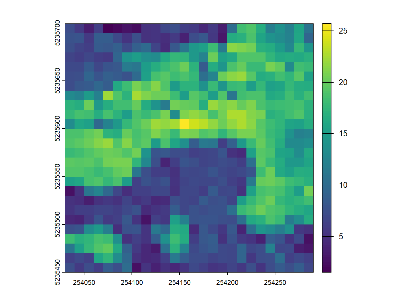

6-LASCATALOG

E1.

Calculate a set of metrics from the lidRmetrics package on the catalogue (voxel metrics will take too long)

Code

ctg <- readLAScatalog(folder = "data/ctg_norm")
dispersion <- pixel_metrics(ctg, ~metrics_dispersion(z = Z, dz = 2, zmax = 30), res = 20)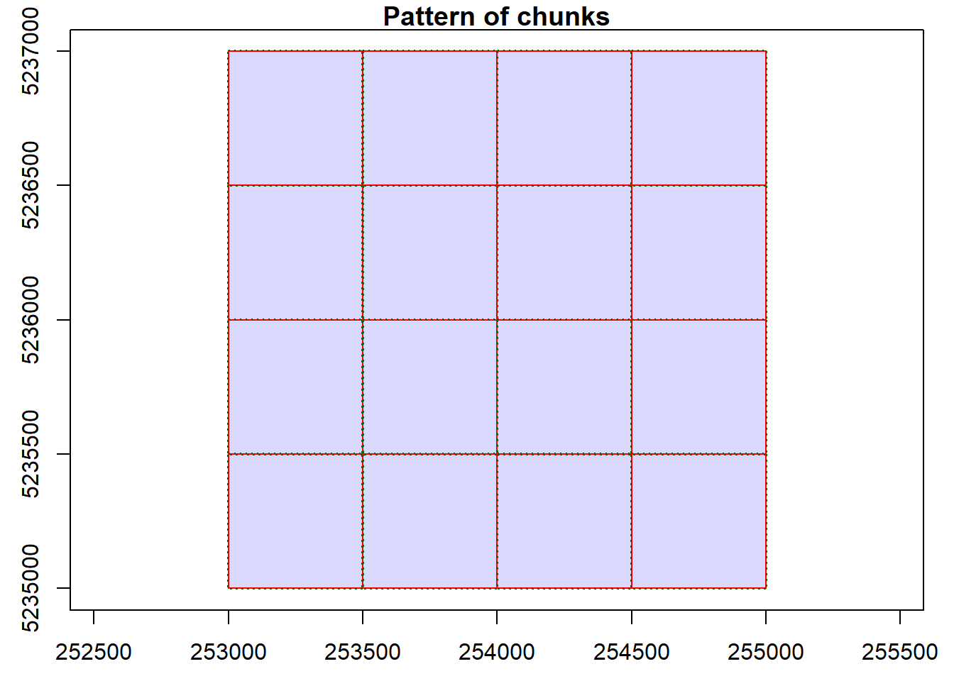

#> Chunk 1 of 16 (6.2%): state ✓
#> 
                                                                                
Chunk 2 of 16 (12.5%): state ✓
#> 
                                                                                
Chunk 3 of 16 (18.8%): state ✓
#> 
                                                                                
Chunk 4 of 16 (25%): state ✓
#> 
                                                                                
Chunk 5 of 16 (31.2%): state ✓
#> 
                                                                                
Chunk 6 of 16 (37.5%): state ✓
#> 
                                                                                
Chunk 7 of 16 (43.8%): state ✓
#> 
                                                                                
Chunk 8 of 16 (50%): state ✓
#> 
                                                                                
Chunk 9 of 16 (56.2%): state ✓
#> 
                                                                                
Chunk 10 of 16 (62.5%): state ✓
#> 
                                                                                
Chunk 11 of 16 (68.8%): state ✓
#> 
                                                                                
Chunk 12 of 16 (75%): state ✓
#> 
                                                                                
Chunk 13 of 16 (81.2%): state ✓
#> 
                                                                                
Chunk 14 of 16 (87.5%): state ✓
#> 
                                                                                
Chunk 15 of 16 (93.8%): state ✓
#> 
                                                                                
Chunk 16 of 16 (100%): state ✓
#> 
                                                                                
plot(dispersion)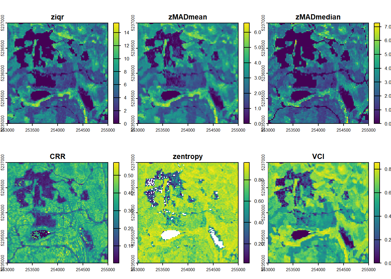

E2.

Read in the non-normalized las catalog filtering the point cloud to only include first returns.

Code

ctg <- readLAScatalog(folder = "data/ctg_class")
opt_filter(ctg) <- "-keep_first -keep_class 2"

E3.

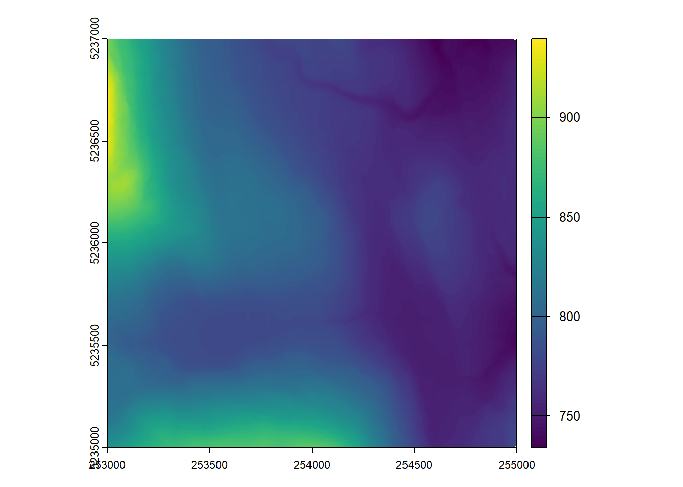
Generate a DTM at 1m spatial resolution for the provided catalog with only first returns.

Code

dtm_first <- rasterize_terrain(ctg, res = 1, algorithm = tin())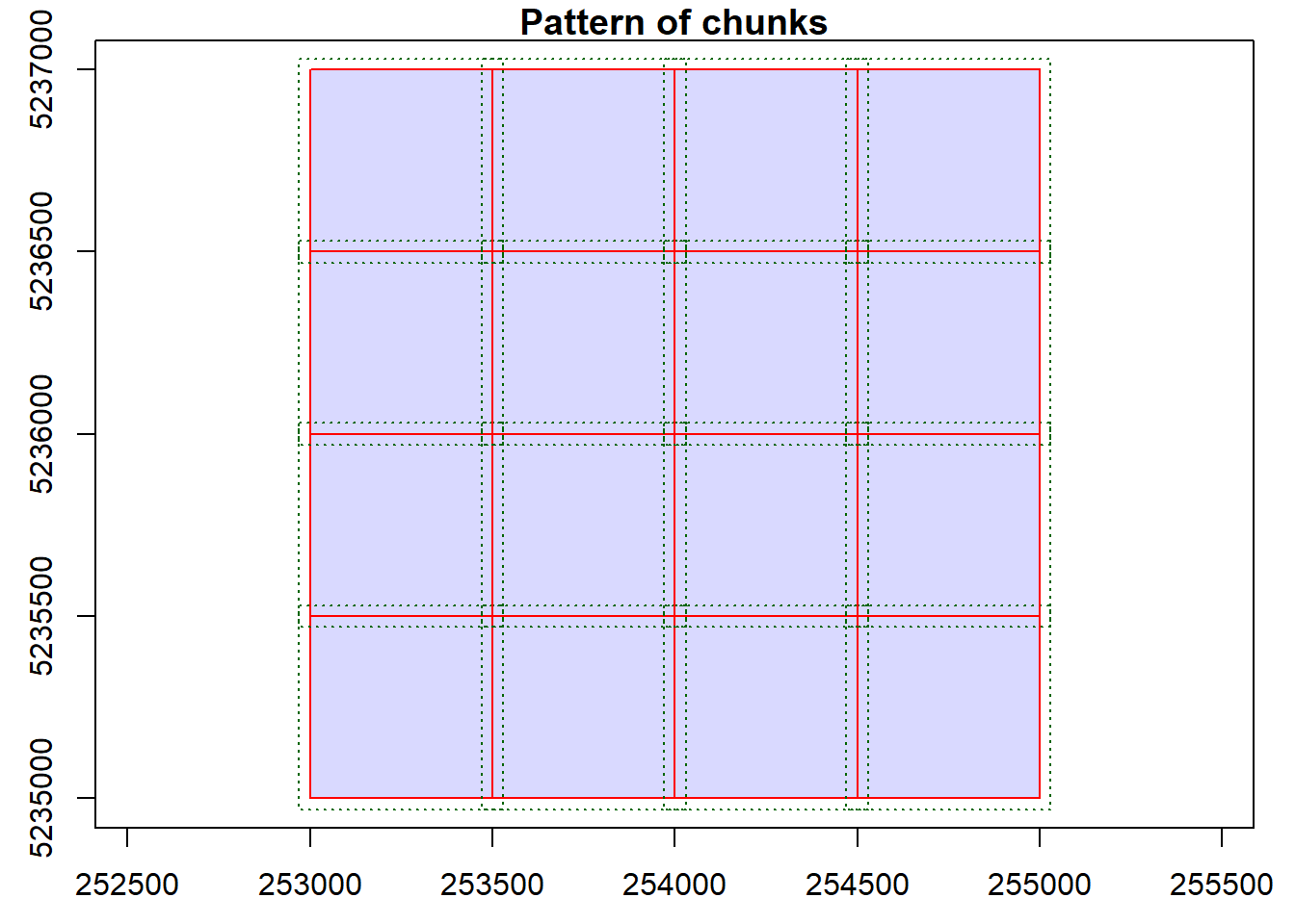

#> Chunk 1 of 16 (6.2%): state ✓
#> 
                                                                                
Chunk 2 of 16 (12.5%): state ✓
#> 
                                                                                
Chunk 3 of 16 (18.8%): state ✓
#> 
                                                                                
Chunk 4 of 16 (25%): state ✓
#> 
                                                                                
Chunk 5 of 16 (31.2%): state ✓
#> 
                                                                                
Chunk 6 of 16 (37.5%): state ✓
#> 
                                                                                
Chunk 7 of 16 (43.8%): state ✓
#> 
                                                                                
Chunk 8 of 16 (50%): state ✓
#> 
                                                                                
Chunk 9 of 16 (56.2%): state ✓
#> 
                                                                                
Chunk 10 of 16 (62.5%): state ✓
#> 
                                                                                
Chunk 11 of 16 (68.8%): state ✓
#> 
                                                                                
Chunk 12 of 16 (75%): state ✓
#> 
                                                                                
Chunk 13 of 16 (81.2%): state ✓
#> 
                                                                                
Chunk 14 of 16 (87.5%): state ✓
#> 
                                                                                
Chunk 15 of 16 (93.8%): state ✓
#> 
                                                                                
Chunk 16 of 16 (100%): state ✓
#> 
                                                                                
plot(dtm_first)