# Clear environment
rm(list = ls(globalenv()))
# Load packages
library(lidR)
library(sf)
library(terra)
library(dplyr)Area-based Approach
Relevant Resources
Overview
The area-based approach (ABA) is a widely-used method for estimating forest attributes, such as timber volume and biomass, by combining field measurements with wall-to-wall lidar data.
Here we will demonstrate a typical implementation of the area-based approach (ABA) for forest attribute estimation using lidar data and ground plot measurements.
Environment
Key References
ABA takes lidar point cloud metrics and connects them (through regression) to forest (or other ecosystem) attributes typically measured on the ground in field plots. This now fundamental approach was originally presented by Nasset 2002.
ABA generally use coregistered plots (measured with GNSS coordinates) as samples to build models to estimate field measured attributes across wall-to-wall coverages of lidar pixel_metrics.
In doing so we can apply models to lidar derived metric rasters over wider coverages to create estimate maps of key forest inventory variables such as stem volume, basal area, and stem density.
knitr::include_graphics("img/white2013_fig4.png")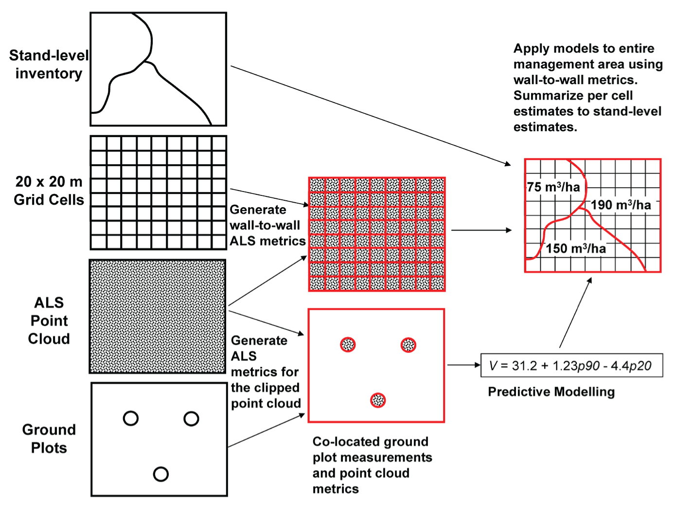
Ground Plot Data
Today we will work will a series of fixed radius (11.28 m) circular plots (n = 162), measured across Forêt Montmorency during 2015 and 2016.
At each of these locations a 400 m2 circular area was established in the field, each tree (above a certain size threshold) was measured and the tree list was processed into metrics describing the merchantable stem volume, stem density, and basal area using regional equations.
Today we will perform the steps necessary to integrate these plot measurements together with coincident ALS data into an area-based prediction of field measured attributes across the wider ALS coverage.
We will focus on the processing of the lidar dataset, and present some very simple model development steps, for more detail on model development and prediction see White 2017.
Plot Level lidar Metrics
Option 1: Integrated plot_metrics function
# Read in plot centres
plots <- st_read("data/plots/ctg_plots.gpkg", quiet = TRUE)
# Read in catalog of normalized LAZ tiles
ctg <- catalog("data/ctg_norm")
plot(st_geometry(ctg@data))
plot(st_geometry(plots ), add = TRUE, col = "red")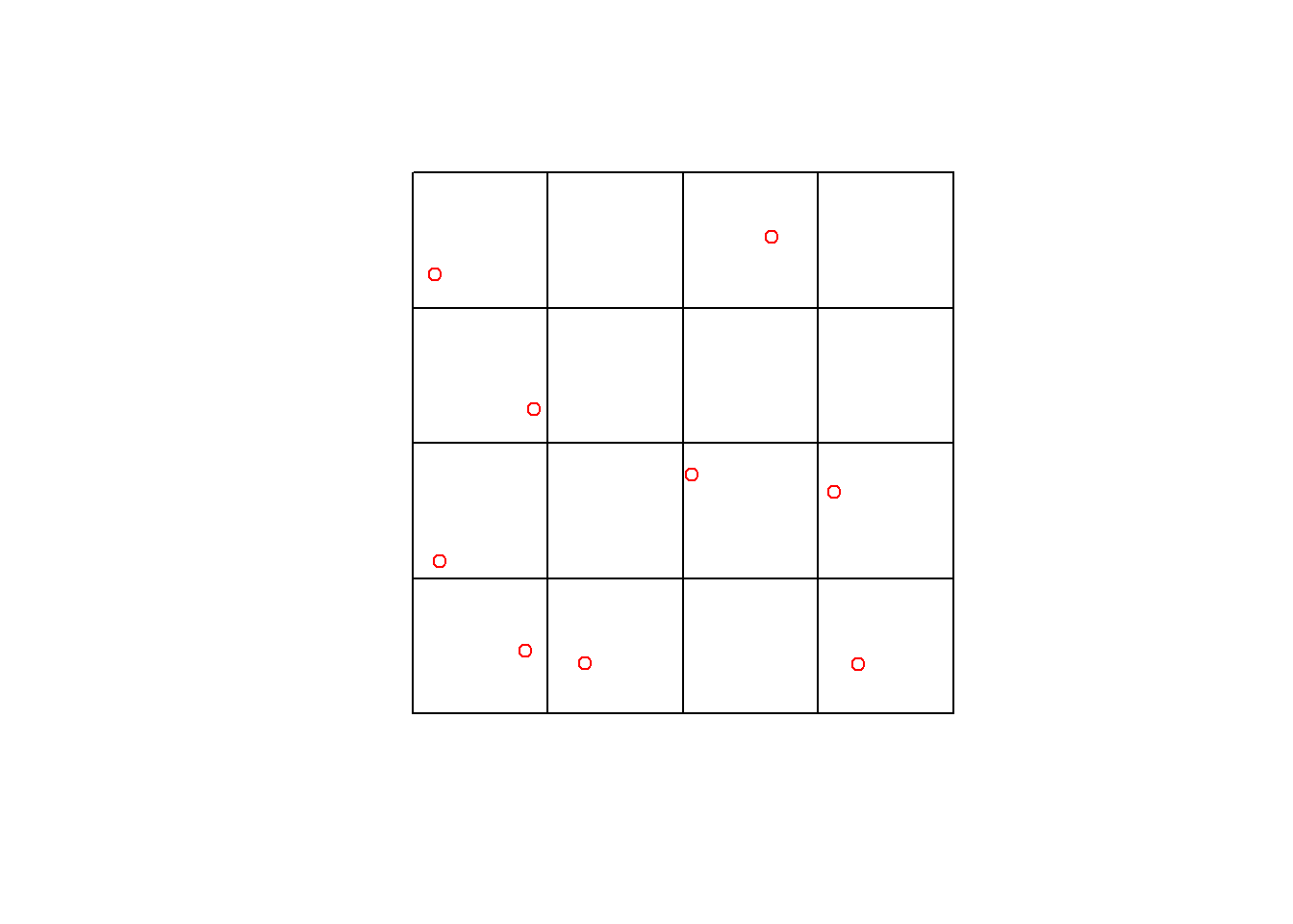
# Calculate with all-in-one plot_metrics function
plot_mets <- plot_metrics(las = ctg, # use the catalog of normalized LAZ files
func = .stdmetrics, # use standard list of metrics
geometry = plots, # use plot centres
radius = 11.28 # define the radius of the circular plots
)
# Select subset of metrics from the resulting dataframe for model development
plot_mets <- dplyr::select(plot_mets,
c(plot_id, ba_ha, sph_ha, # forest attributes
merch_vol_ha, zq95, pzabove2, zskew # lidar metrics
))
plot_mets
#> Simple feature collection with 9 features and 7 fields
#> Geometry type: POINT
#> Dimension: XY
#> Bounding box: xmin: 253081.7 ymin: 5235181 xmax: 254649 ymax: 5236762
#> Projected CRS: NAD83(CSRS) / MTM zone 7
#> plot_id ba_ha sph_ha merch_vol_ha zq95 pzabove2 zskew
#> 1 9909900501 1.486 100 8.115642 6.9000 81.55102 -0.49723746
#> 2 9909900601 8.375 450 47.981479 8.7600 68.73385 0.27413450
#> 3 9909900901 31.983 1675 183.184410 12.2415 70.30217 -0.19735942
#> 4 7100603001 23.375 916 146.121568 10.7010 69.13793 -0.10241971
#> 5 9909900401 32.748 2125 170.614048 11.4000 69.61451 -0.28367425
#> 6 9909900801 8.759 475 44.052570 7.2320 64.66711 0.20208907
#> 7 9809902401 34.636 1466 209.197220 14.5860 76.99065 -0.01132556
#> 8 9809902901 22.081 1075 132.254507 10.7610 57.11733 0.59273314
#> 9 9809902701 25.772 1332 158.900586 11.8100 78.99215 0.23885411
#> geom
#> 1 POINT (253417.9 5235232)
#> 2 POINT (253100.3 5235562)
#> 3 POINT (253446.8 5236125)
#> 4 POINT (253081.7 5236624)
#> 5 POINT (253637.7 5235185)
#> 6 POINT (254032.3 5235882)
#> 7 POINT (254327 5236762)
#> 8 POINT (254649 5235181)
#> 9 POINT (254558 5235820)Option 2: clip_roi and catalog_apply
While the plot_metrics function is efficient, you may want more control over the process or wish to save the point clouds for each plot for further analysis. The following code demonstrates a more manual workflow. First, we will clip the lidar point clouds using the plot boundaries and save each clipped plot as a separate .laz file. We then create a new catalog of these individual plot point clouds and use catalog_apply to calculate standard metrics for each point cloud.
Now we will clip the circular plots, save them as .laz files, and treat them as a catalog of independent lidar files to calculate a table of metrics.
# Clip normalized LAZ files for each plot location
opt_output_files(ctg) <- "data/plots/las/{plot_id}"
opt_laz_compression(ctg) <- TRUE
# Create circular polygons of 11.28m radius (400m2 area)
plot_buffer <- st_buffer(plots, 11.28)
# Clip normalized LAZ file for each plot
clip_roi(ctg, plot_buffer)#> class : LAScatalog (v1.2 format 1)
#> extent : 253070.5, 254660.2, 5235170, 5236773 (xmin, xmax, ymin, ymax)
#> coord. ref. : NAD83(CSRS) / MTM zone 7
#> area : 4480.351 m²
#> points : 16.8 thousand points
#> type : airborne
#> density : 3.8 points/m²
#> density : 2.8 pulses/m²
#> num. files : 9This resulting folder of individual plot .laz files can now be treated as a catalog of independent files to generate a table of metrics.
# Create a new catalog referencing the clipped plots we saved
ctg_plot <- catalog("data/plots/las")
opt_independent_files(ctg_plot) <- TRUE # process each plot independently
# Define a metrics function to apply to plots
generate_plot_metrics <- function(chunk){
# Check if tile is empty
las <- readLAS(chunk)
if (is.empty(las)) return(NULL)
# Calculate standard list of metrics (56) built in to lidR for each point cloud
mets <- cloud_metrics(las, .stdmetrics)
# Convert output metrics to dataframe (from list)
mets_df <- as.data.frame(mets)
# Add plot ID to metrics dataframe
mets_df$plot_id <- gsub(basename(chunk@files),
pattern = ".laz",
replacement = "")
return(mets_df)
}
# Apply our function to each plot in the catalog
plot_mets <- catalog_apply(ctg_plot, generate_plot_metrics)
# Bind the output dataframes into one table
plot_df <- do.call(rbind, plot_mets)
# Rejoin the lidar metrics with the plot vector with attributes
plot_sf <- left_join(plots, plot_df, by = "plot_id")
# Select subset of metrics for model development
plot_mets <- dplyr::select(plot_sf,
c(plot_id, ba_ha, sph_ha, # forest attributes
merch_vol_ha, zq95, pzabove2, zskew # lidar metrics
))
plot_mets
#> Simple feature collection with 9 features and 7 fields
#> Geometry type: POINT
#> Dimension: XY
#> Bounding box: xmin: 253081.7 ymin: 5235181 xmax: 254649 ymax: 5236762
#> Projected CRS: NAD83(CSRS) / MTM zone 7
#> plot_id ba_ha sph_ha merch_vol_ha zq95 pzabove2 zskew
#> 1 9909900501 1.486 100 8.115642 6.9000 81.55102 -0.49723746
#> 2 9909900601 8.375 450 47.981479 8.7600 68.73385 0.27413450
#> 3 9909900901 31.983 1675 183.184410 12.2420 70.28814 -0.19650975
#> 4 7100603001 23.375 916 146.121568 10.7020 69.16774 -0.10322875
#> 5 9909900401 32.748 2125 170.614048 11.4000 69.65400 -0.28490728
#> 6 9909900801 8.759 475 44.052570 7.2320 64.66711 0.20208907
#> 7 9809902401 34.636 1466 209.197220 14.5865 76.98413 -0.01112273
#> 8 9809902901 22.081 1075 132.254507 10.7615 57.09178 0.59437401
#> 9 9809902701 25.772 1332 158.900586 11.8100 79.04388 0.23861734
#> geom
#> 1 POINT (253417.9 5235232)
#> 2 POINT (253100.3 5235562)
#> 3 POINT (253446.8 5236125)
#> 4 POINT (253081.7 5236624)
#> 5 POINT (253637.7 5235185)
#> 6 POINT (254032.3 5235882)
#> 7 POINT (254327 5236762)
#> 8 POINT (254649 5235181)
#> 9 POINT (254558 5235820)What we are left with is a dataframe of plot-level lidar metrics and field measured forest attributes that we can use to develop predictive models for wall-to-wall mapping.
Applying across Forêt Montmorency
Plot Network
Model Development
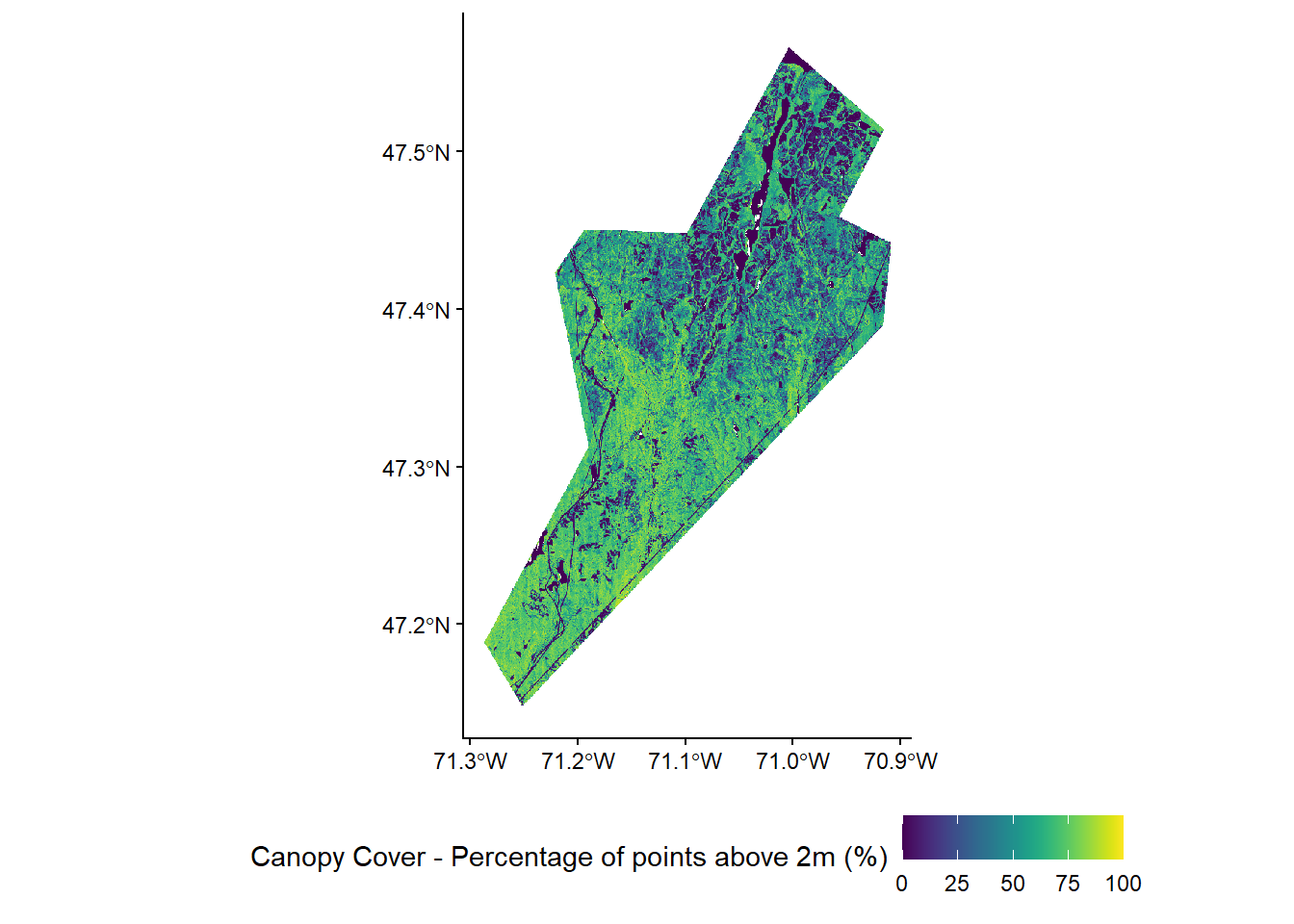
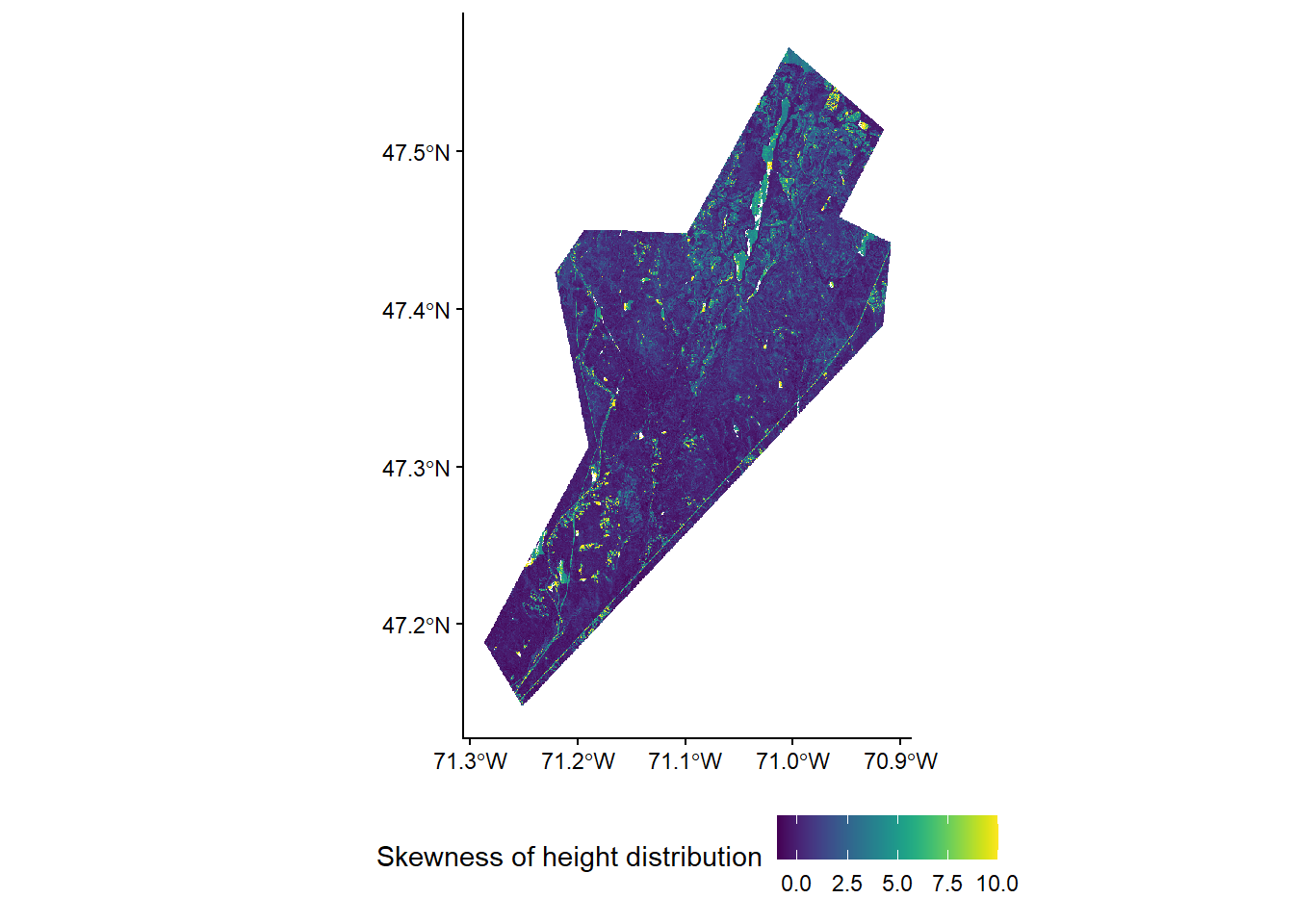
To keep things simple we will use a small set of three lidar metrics that are commonly used in ABA models: - zq95 - 95th percentile of height (canopy height) - pzabove2 - Percentage of points above 2m (canopy cover) - zskew - Skewness of the height distribution (height variability)
For more information read: White 2017
We will generate simple linear models for each of our three forest attributes using these three lidar metrics as predictors and our 169 field plots as samples.
knitr::include_graphics("img/white2017_fig3.png")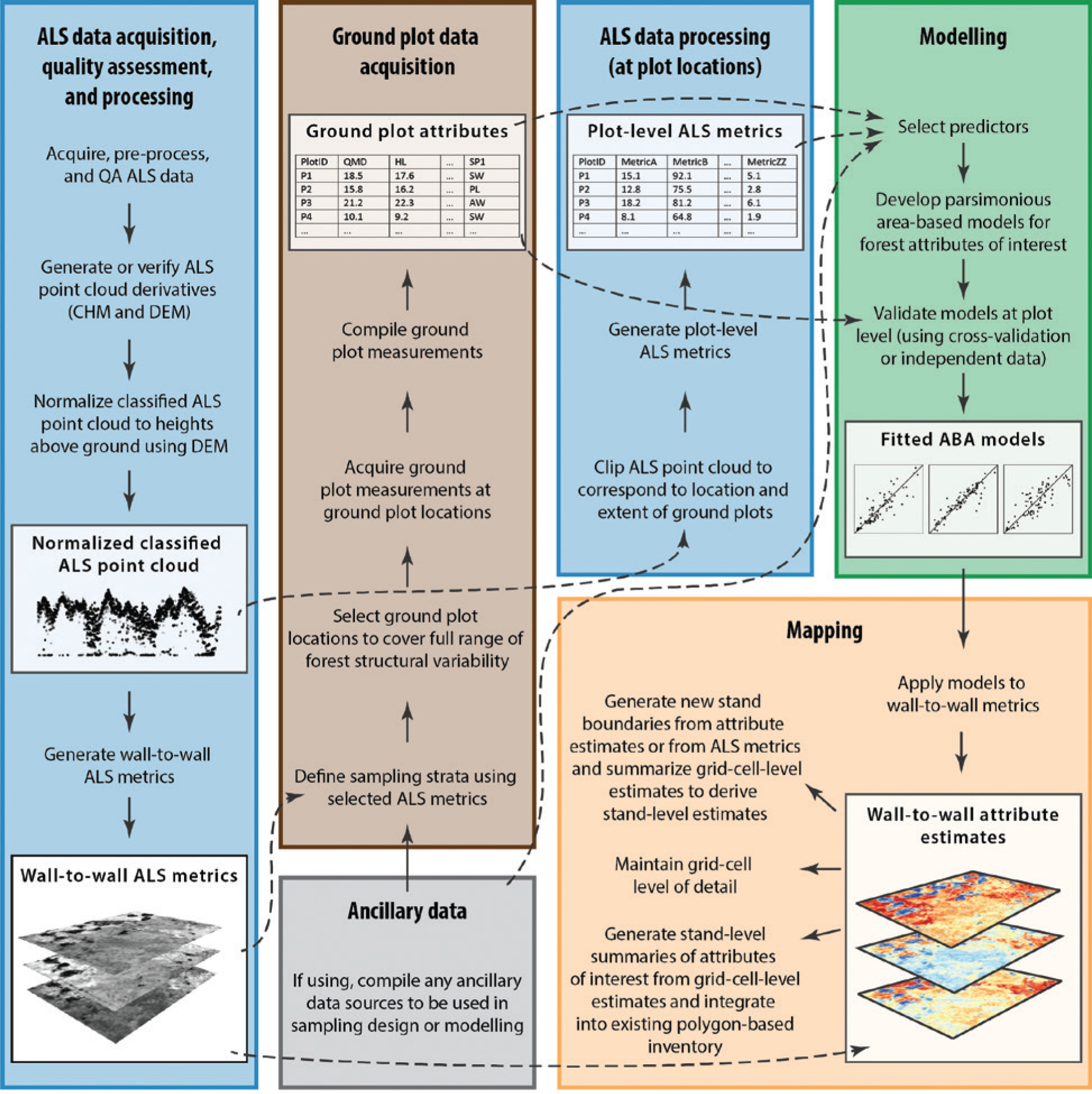
# Read in plot metrics with forest attributes and lidar metrics calculated for all 162 plots
plot_mets <- read.csv("data/plots/plots_all.csv")
# Generate linear models for each forest attribute using three lidar metrics
lm_vol <- lm(merch_vol_ha ~ zq95 + zskew + pzabove2, data = plot_mets)
lm_ba <- lm(ba_ha ~ zq95 + zskew + pzabove2, data = plot_mets)
lm_sph <- lm(sph_ha ~ zq95 + zskew + pzabove2, data = plot_mets)
# Extract model coefficients
vol_cf <- lm_vol$coefficients
ba_cf <- lm_ba$coefficients
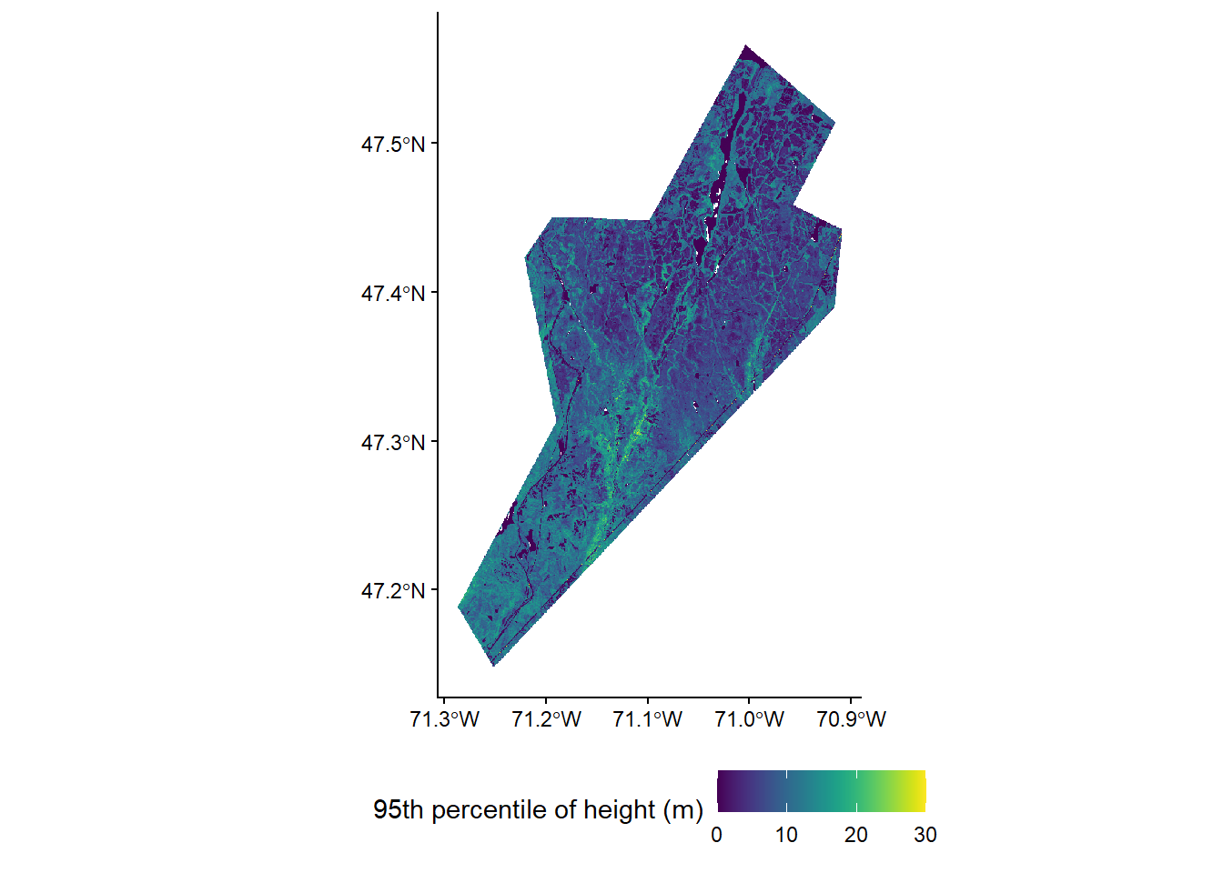
sph_cf <- lm_sph$coefficientsNow that we have our models, we can apply them to wall-to-wall lidar metrics calculated across the entire Forêt Montmorency. These metrics have been pre-computed from the larger ALS catalog coverage of 160,000 hectares in area.
Non-Forest Mask
Before applying our predictive models, it is important to mask out non-forest areas (e.g. roads, water bodies, unsampled forest types) from our wall-to-wall metrics. Applying models trained on forest plots to non-forest pixels will produce spurious predictions.White et al. 2013 (Section 4.4.1)
In this example our forest mask is a polygon representing forested land cover, pixels falling outside this polygon are set to NA.
Beneath each masked raster, observe how the ‘population’ of pixel metric values changes following this critical step.
Download the forest mask (.gpkg, 4.1 MB)
# Read forest mask polygon
forest_mask <- vect("data/forest_mask.gpkg")
# Apply the mask directly - pixels outside the forest polygon become NA
metrics_masked <- mask(metrics_rast, forest_mask)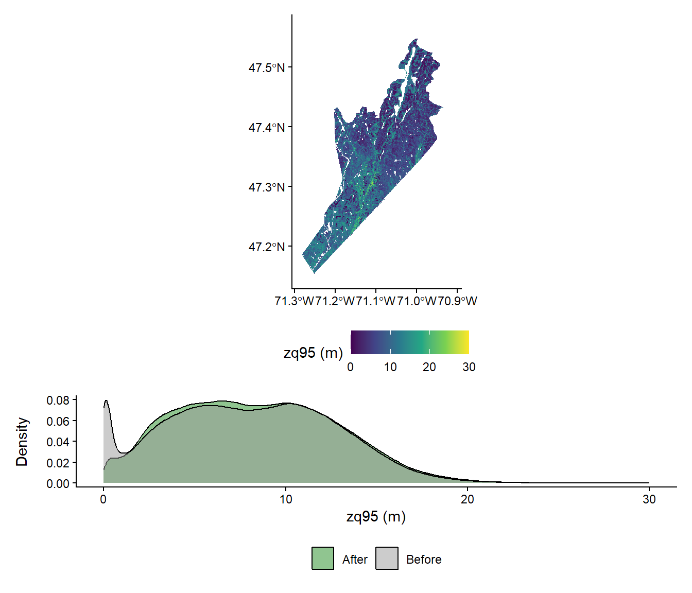
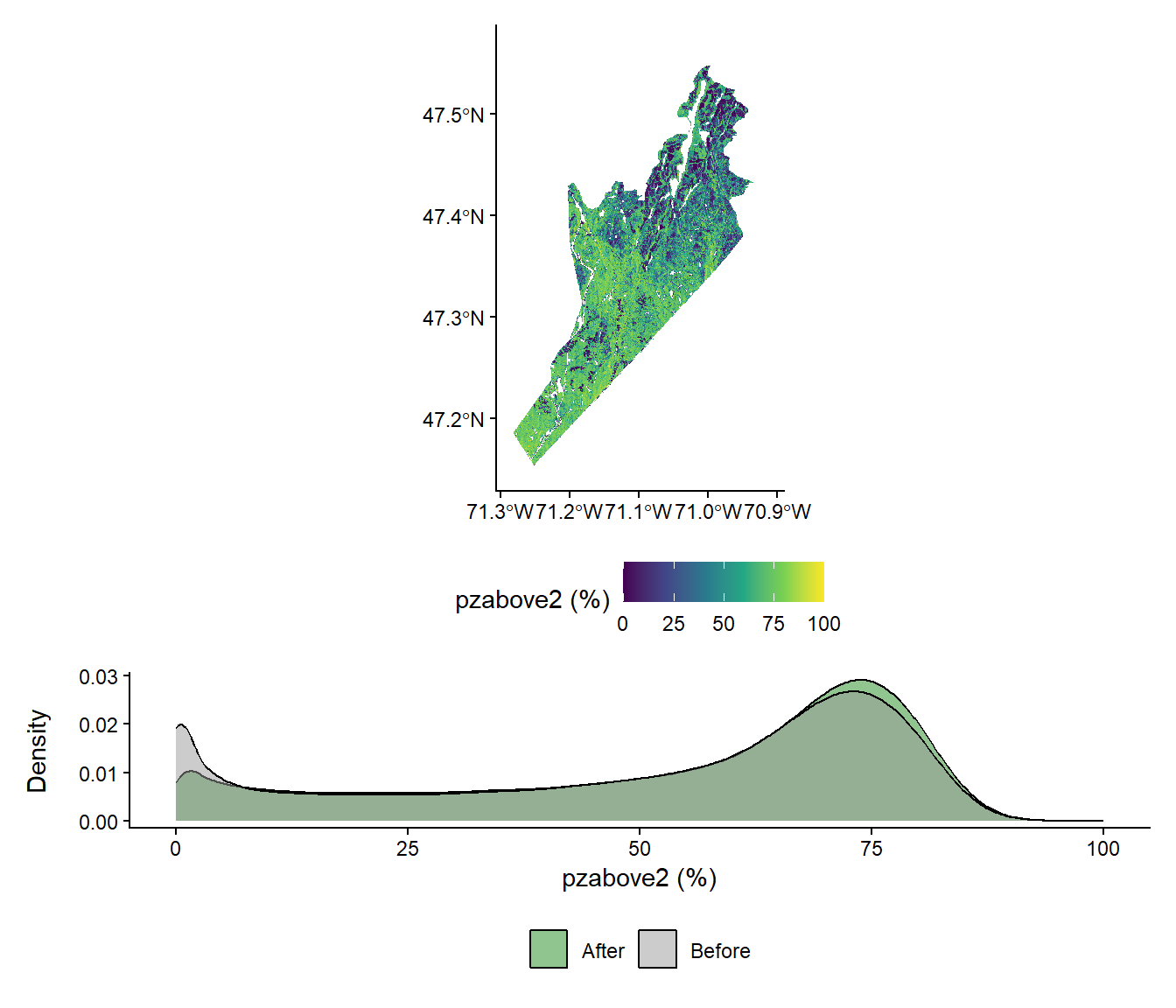
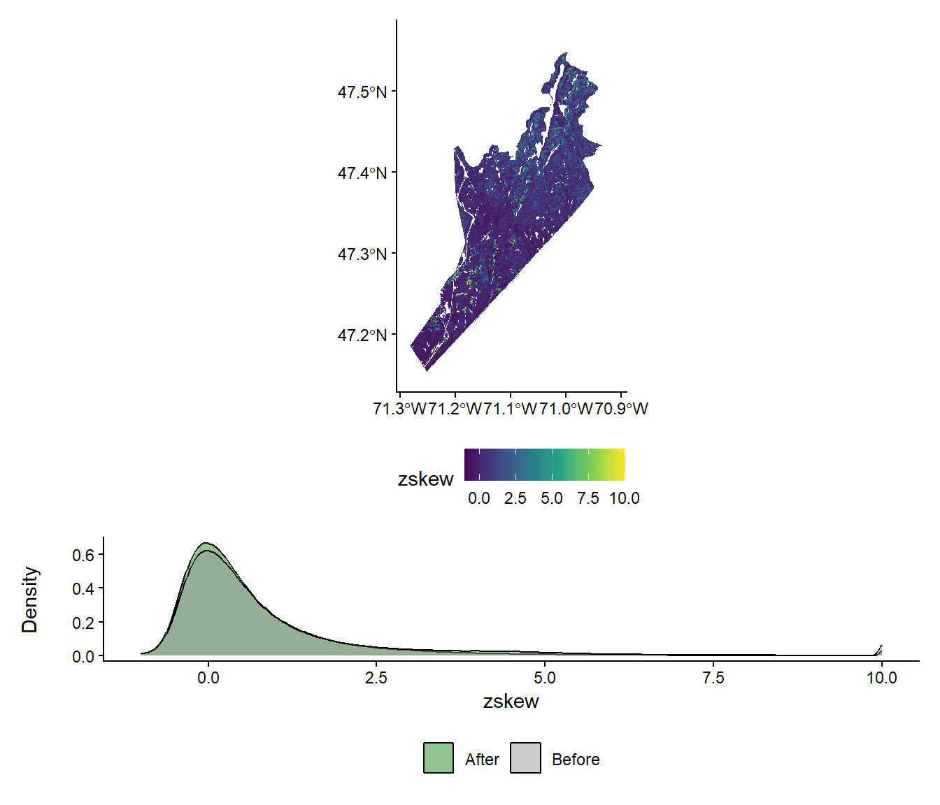
After masking, we replace our original metrics raster with the masked version for all subsequent model application steps.
# Use masked metrics for model application
metrics_rast <- metrics_maskedApplying Models
To apply our models we need to create wrapper functions that take our model coefficients and apply them to our pixel metric raster layers.
We will create functions that follows the standard lm formula: y = b0 + b1x1 + b2x2 + b3*x3
Where y is the attribute, b0 is the intercept, b1, b2, and b3 are the coefficients
Here we will create three functions, one for each of our forest attributes: Stem Volume (m3/ha), Basal Area (m2/ha), and Stem Density (stems/ha).
# Create functions from model coefficients that we can apply to metrics rasters
# Function to predict stem volume
vol_lm_r <- function(zq95,zskew,pzabove2){
vol_cf["(Intercept)"] + (vol_cf["zq95"] * zq95) + (vol_cf["zskew"] * zskew) + (vol_cf["pzabove2"] * pzabove2)
}
# Function to predict basal area
ba_lm_r <- function(zq95,zskew,pzabove2){
ba_cf["(Intercept)"] + (ba_cf["zq95"] * zq95) + (ba_cf["zskew"] * zskew) + (ba_cf["pzabove2"] * pzabove2)
}
# Function to predict stem density
sph_lm_r <- function(zq95,zskew,pzabove2){
sph_cf["(Intercept)"] + (sph_cf["zq95"] * zq95) + (sph_cf["zskew"] * zskew) + (sph_cf["pzabove2"] * pzabove2)
}In this example we will achieve this using the terra package with the lapp function that will apply our function to the wall-to-wall metrics raster to generate maps of our three forest attributes. lapp applies a function to each cell of our multi-layer metric raster.
plot(metrics_rast)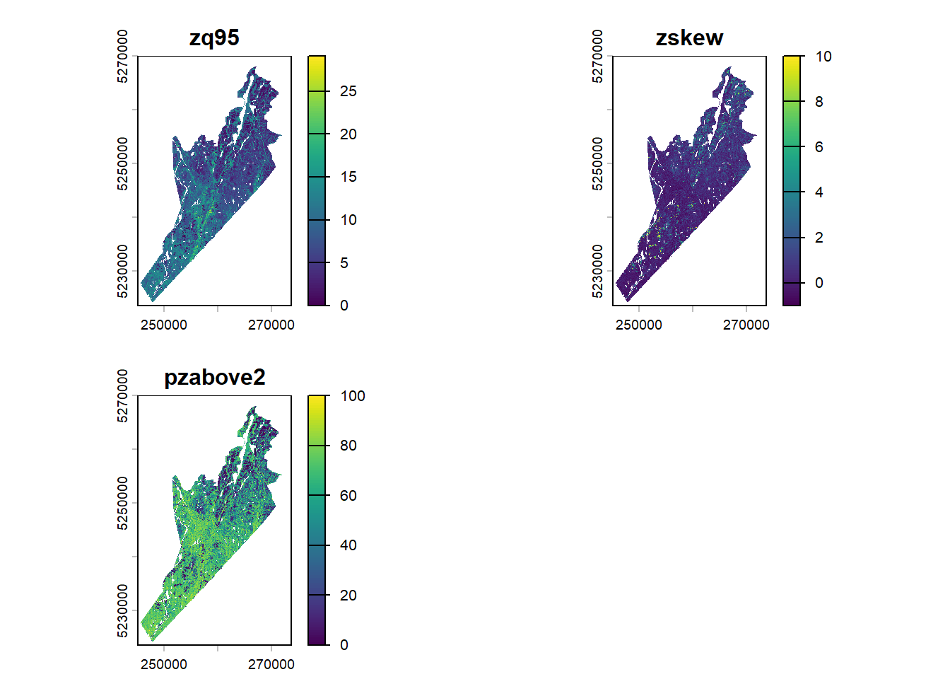
# Apply models to generate wall-to-wall forest attribute estimates
# Merchantable Stem Volume
vol_r <- terra::lapp(metrics_rast, fun = vol_lm_r)
plot(vol_r, main = "Merchantable Stem Volume (m3/ha)")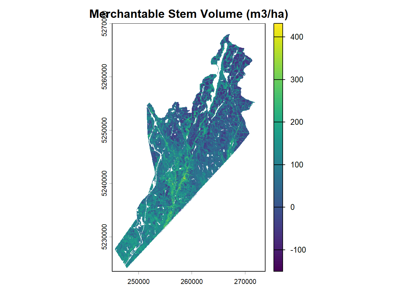
# Basal Area
ba_r <- terra::lapp(metrics_rast, fun = ba_lm_r)
plot(ba_r, main = "Basal Area (m2/ha)")
# Stem Density
sph_r <- terra::lapp(metrics_rast, fun = sph_lm_r)
plot(sph_r, main = "Stem Density (stems/ha)")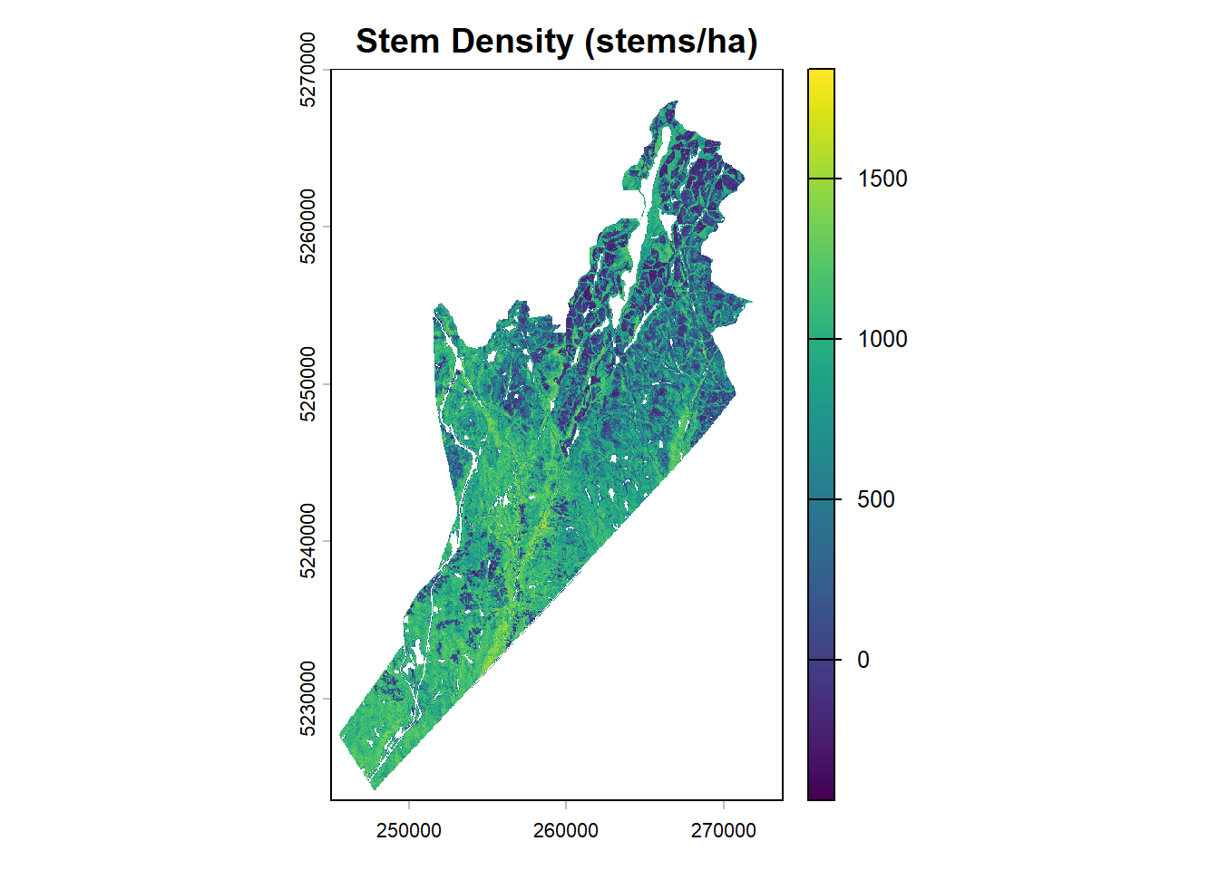
Conclusion
We have demonstrated the area-based approach (ABA) for estimating forest attributes using lidar data and ground plot measurements. By calculating plot-level lidar metrics and developing predictive models, we can generate wall-to-wall maps of key forest inventory variables such as stem volume, basal area, and stem density.
Here we used simple linear models for demonstration purposes, but more advanced modeling techniques can be employed such as random forest models.