# Clear environment
rm(list = ls(globalenv()))

# Load packages
library(lidR)
library(sf)
library(terra)
library(dplyr)Regions of Interest (ROI)
Relevant Resources
Overview
The area-based approach (ABA) is a widely-used method for estimating forest attributes, such as timber volume and biomass, by combining field measurements with wall-to-wall lidar data.
Here we will demonstrate a typical implementation of the area-based approach (ABA) for forest attribute estimation using lidar data and ground plot measurements.
In this section we demonstrate the selection of regions of interest (ROIs) from lidar data using simple geometries (circles) and geometries extracted from shapefiles.
Environment
Simple Geometries
Load lidar Data and Inspect
We start by loading some lidar data and inspecting its header and number of point records.
las <- readLAS(files = 'data/fm_norm.laz')# Inspect the header and the number of point records
las@header
#> File signature: LASF
#> File source ID: 0
#> Global encoding:
#> - GPS Time Type: Standard GPS Time
#> - Synthetic Return Numbers: no
#> - Well Know Text: CRS is WKT
#> - Aggregate Model: false
#> Project ID - GUID: 00000000-0000-0000-0000-000000000000
#> Version: 1.2
#> System identifier:
#> Generating software: rlas R package
#> File creation d/y: 0/0
#> header size: 227
#> Offset to point data: 1319
#> Num. var. length record: 1
#> Point data format: 1
#> Point data record length: 28
#> Num. of point records: 266472
#> Num. of points by return: 204452 51967 9452 593 8
#> Scale factor X Y Z: 0.01 0.01 0.01
#> Offset X Y Z: 2e+05 5200000 0
#> min X Y Z: 254034.6 5235452 -1.83
#> max X Y Z: 254284.6 5235702 23.83
#> Variable Length Records (VLR):
#> Variable Length Record 1 of 1
#> Description: by LAStools of rapidlasso GmbH
#> WKT OGC COORDINATE SYSTEM: PROJCRS["NAD83(CSRS) / MTM zone 7",BASEGEOGCRS["NAD83(CSRS)",DATUM["NA [...] (truncated)
#> Extended Variable Length Records (EVLR): void
las@header$`Number of point records`
#> [1] 266472Select Circular and Rectangular Areas
We can select circular and rectangular areas from the lidar data based on specified coordinates and radii or dimensions.
# Establish coordinates
x <- 254250
y <- 5235510

# Select a circular area
circle <- clip_circle(las = las, xcenter = x, ycenter = y, radius = 30)

# Inspect the circular area and the number of point records
circle
#> class        : LAS (v1.2 format 1)
#> memory       : 605.6 Kb
#> extent       : 254220.1, 254279.9, 5235480, 5235540 (xmin, xmax, ymin, ymax)
#> coord. ref.  : NAD83(CSRS) / MTM zone 7
#> area         : 2790 m²
#> points       : 11 thousand points
#> type         : airborne
#> density      : 3.94 points/m²
#> density      : 2.73 pulses/m²
circle@header$`Number of point records`
#> [1] 10995
# Plot the circular area
plot(circle)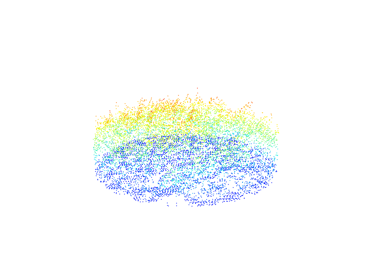
We can do the same with a rectangular area by defining corner coordinates.
# Select a rectangular area
rect <- clip_rectangle(las = las, xleft = x, ybottom = y, xright = x + 40, ytop = y + 30)
# Plot the rectangular area
plot(rect)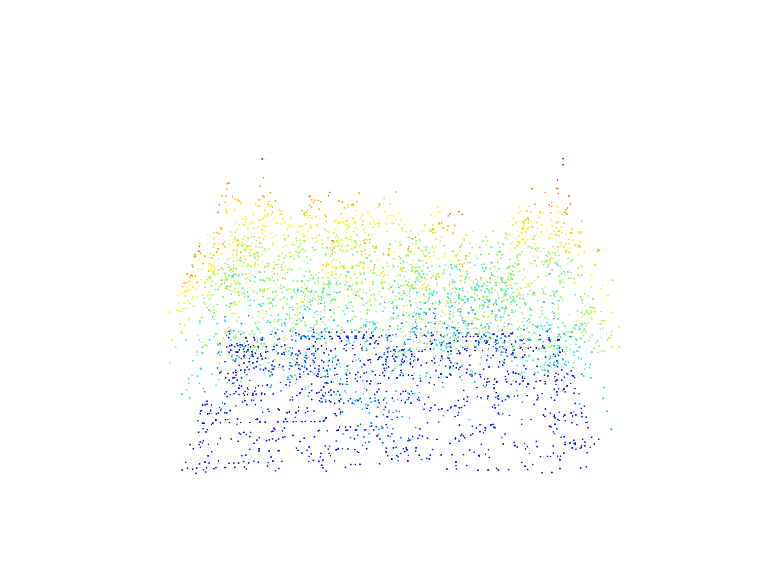
We can also supply multiple coordinate pairs to clip multiple ROIs.
# Select multiple random circular areas
x <- runif(2, x, x)
y <- runif(2, 5235500, 5235700)

plots <- clip_circle(las = las, xcenter = x, ycenter = y, radius = 10)
# Plot each of the multiple circular areas
plot(plots[[1]])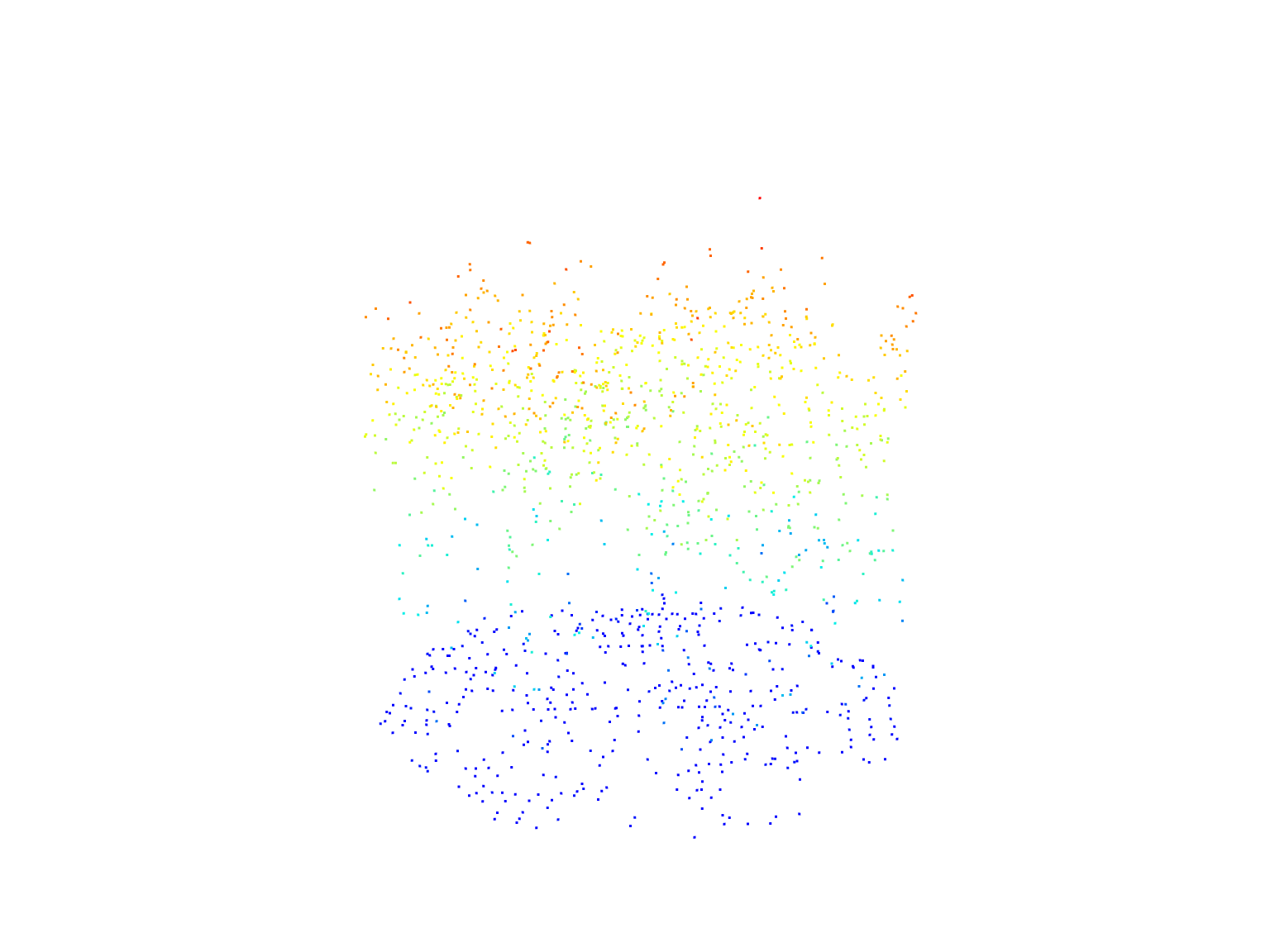
# Plot each of the multiple circular areas
plot(plots[[2]])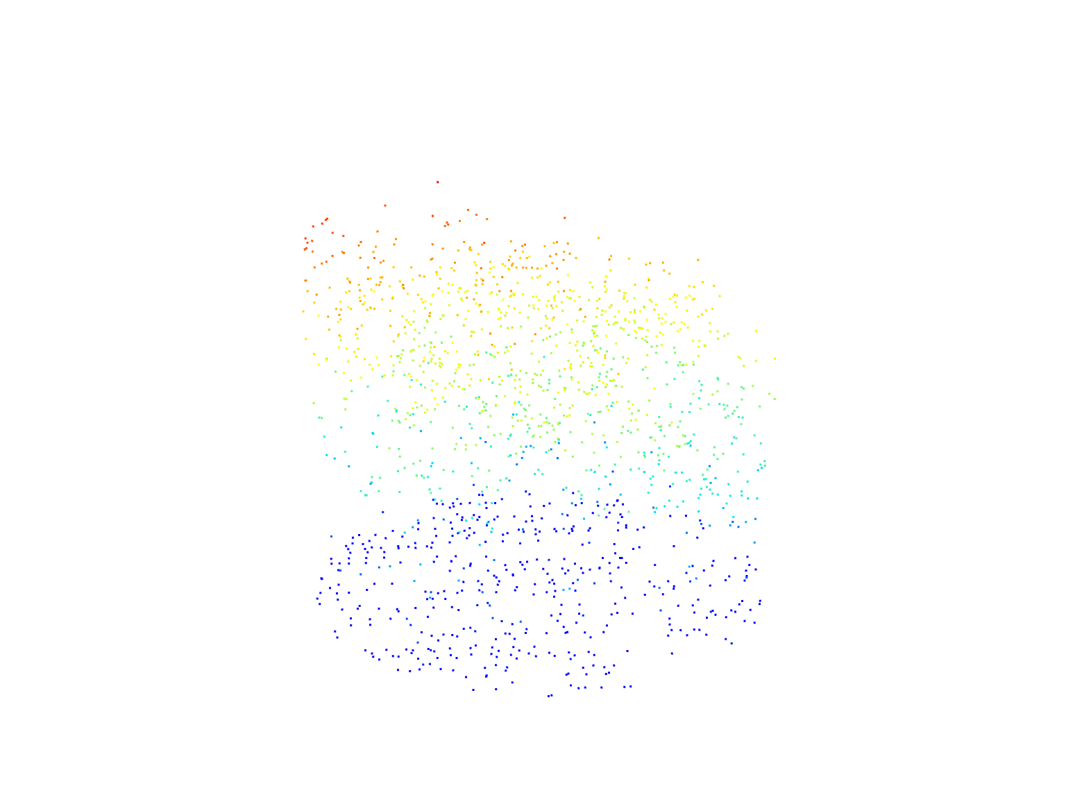
Extraction of Complex Geometries from Shapefiles
We demonstrate how to extract complex geometries from shapefiles using the clip_roi() function from the lidR package.
We use the sf package to load an ROI and then clip to its extents.
# Load the geopackage using sf
stand_bdy <- sf::st_read(dsn = "data/roi/roi.gpkg", quiet = TRUE)

# Plot the lidar header information without the map
plot(las@header, map = FALSE)

# Plot the stand boundary areas on top of the lidar header plot
plot(stand_bdy, add = TRUE, col = "#08B5FF39")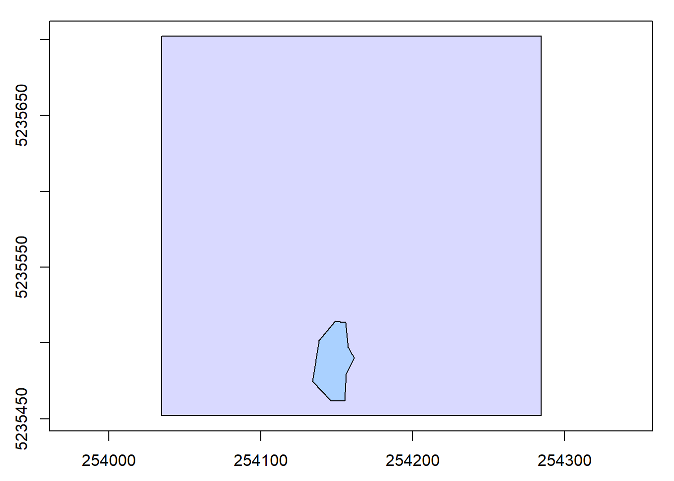
# Extract points within the stand boundary using clip_roi()
stand <- clip_roi(las = las, geometry = stand_bdy)
# Plot the extracted points within the planting areas
plot(stand)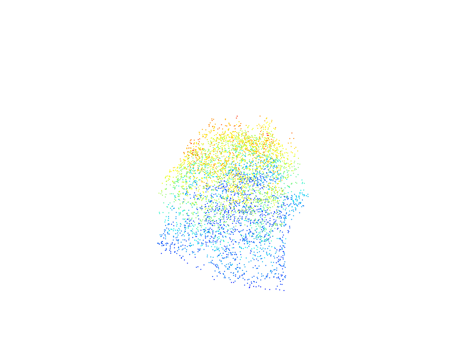
Clipping ROIs with a catalog
We clip the LAS data in the catalog using specified coordinate groups.
ctg <- catalog("data/ctg_norm")

# Set coordinate groups
x <- c(254000, 254250, 254500, 254750, 254780)
y <- c(5235000, 5235250, 5235500, 5235750, 5235800)

# Visualize coordinate groups
plot(ctg)
points(x, y)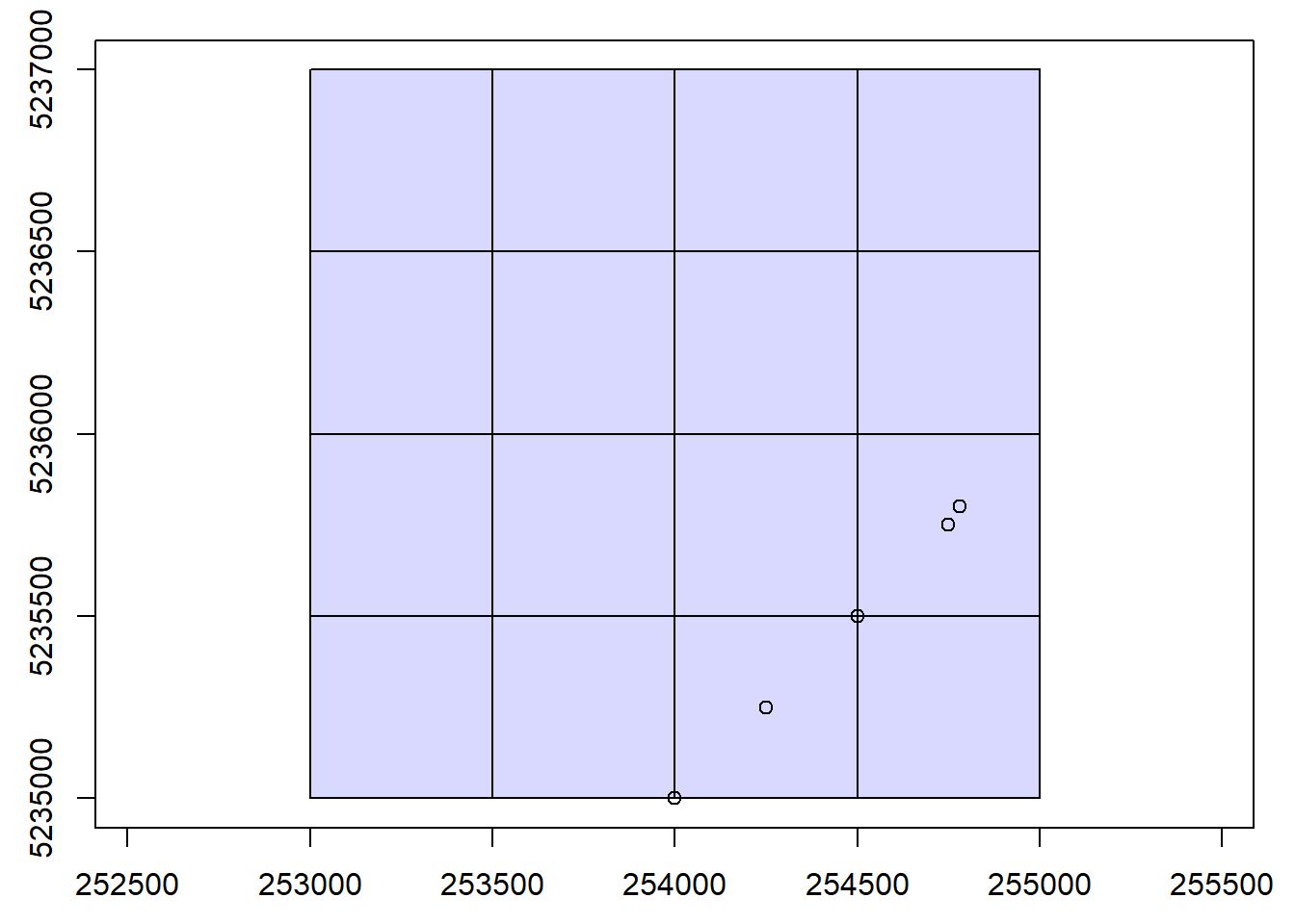
# Clip 30 m plots
rois <- clip_circle(las = ctg, xcenter = x, ycenter = y, radius = 30)plot(rois[[1]])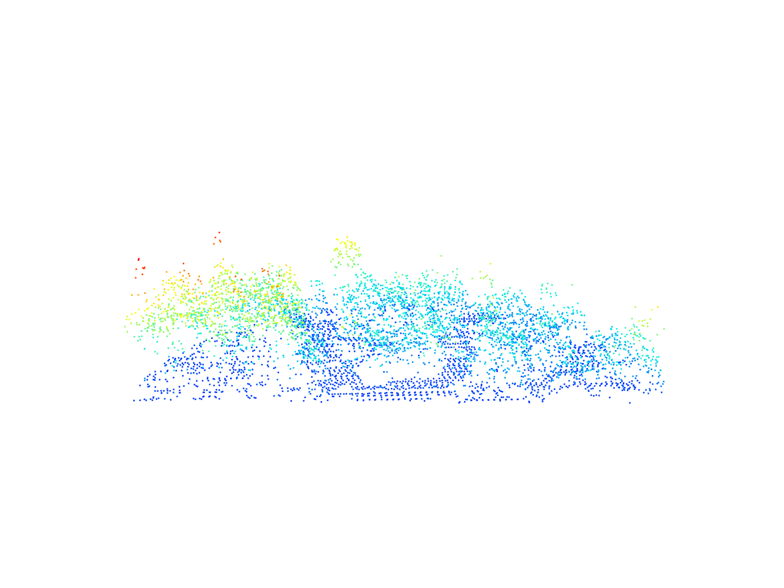
plot(rois[[3]])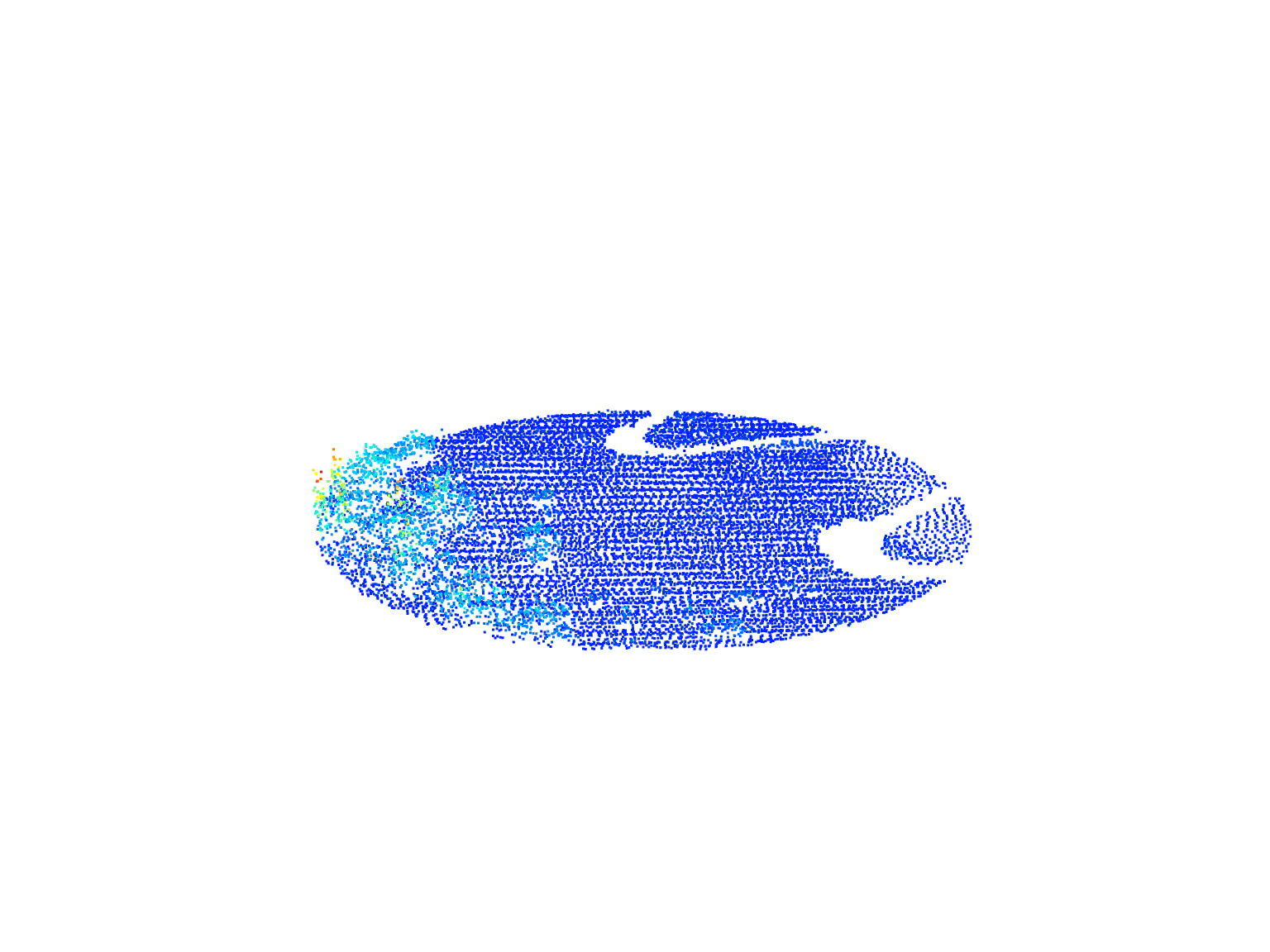
Validate clipped data
We validate the clipped LAS data using the las_check function.
las_check(rois[[1]])
#>
#>  Checking the data
#>   - Checking coordinates... ✓
#>   - Checking coordinates type... ✓
#>   - Checking coordinates range... ✓
#>   - Checking coordinates quantization... ✓
#>   - Checking attributes type... ✓
#>   - Checking ReturnNumber validity... ✓
#>   - Checking NumberOfReturns validity... ✓
#>   - Checking ReturnNumber vs. NumberOfReturns... ✓
#>   - Checking RGB validity... ✓
#>   - Checking absence of NAs... ✓
#>   - Checking duplicated points... ✓
#>   - Checking degenerated ground points... ✓
#>   - Checking attribute population...
#>     🛈 'ScanDirectionFlag' attribute is not populated
#>     🛈 'EdgeOfFlightline' attribute is not populated
#>   - Checking gpstime incoherances ✓
#>   - Checking flag attributes... ✓
#>   - Checking user data attribute...
#>     🛈 5724 points have a non 0 UserData attribute. This probably has a meaning
#>  Checking the header
#>   - Checking header completeness... ✓
#>   - Checking scale factor validity... ✓
#>   - Checking point data format ID validity... ✓
#>   - Checking extra bytes attributes validity... ✓
#>   - Checking the bounding box validity... ✓
#>   - Checking coordinate reference system... ✓
#>  Checking header vs data adequacy
#>   - Checking attributes vs. point format... ✓
#>   - Checking header bbox vs. actual content... ✓
#>   - Checking header number of points vs. actual content... ✓
#>   - Checking header return number vs. actual content... ✓
#>  Checking coordinate reference system...
#>   - Checking if the CRS was understood by R... ✓
#>  Checking preprocessing already done
#>   - Checking ground classification... yes
#>   - Checking normalization... maybe
#>   - Checking negative outliers...
#>     ⚠ 224 points below 0
#>   - Checking flightline classification... yes
#>  Checking compression
#>   - Checking attribute compression...
#>    -  ScanDirectionFlag is compressed
#>    -  EdgeOfFlightline is compressed
#>    -  Synthetic_flag is compressed
#>    -  Keypoint_flag is compressed
#>    -  Withheld_flag is compressed
#>    -  UserData is compressed
#>    -  PointSourceID is compressed
las_check(rois[[3]])
#>
#>  Checking the data
#>   - Checking coordinates... ✓
#>   - Checking coordinates type... ✓
#>   - Checking coordinates range... ✓
#>   - Checking coordinates quantization... ✓
#>   - Checking attributes type... ✓
#>   - Checking ReturnNumber validity... ✓
#>   - Checking NumberOfReturns validity... ✓
#>   - Checking ReturnNumber vs. NumberOfReturns... ✓
#>   - Checking RGB validity... ✓
#>   - Checking absence of NAs... ✓
#>   - Checking duplicated points... ✓
#>   - Checking degenerated ground points...
#>     ⚠ There were 3 degenerated ground points. Some X Y coordinates were repeated but with different Z coordinates
#>   - Checking attribute population...
#>     🛈 'ScanDirectionFlag' attribute is not populated
#>     🛈 'EdgeOfFlightline' attribute is not populated
#>   - Checking gpstime incoherances
#>     ✗ 1673 pulses (points with the same gpstime) have points with identical ReturnNumber
#>   - Checking flag attributes... ✓
#>   - Checking user data attribute...
#>     🛈 16015 points have a non 0 UserData attribute. This probably has a meaning
#>  Checking the header
#>   - Checking header completeness... ✓
#>   - Checking scale factor validity... ✓
#>   - Checking point data format ID validity... ✓
#>   - Checking extra bytes attributes validity... ✓
#>   - Checking the bounding box validity... ✓
#>   - Checking coordinate reference system... ✓
#>  Checking header vs data adequacy
#>   - Checking attributes vs. point format... ✓
#>   - Checking header bbox vs. actual content... ✓
#>   - Checking header number of points vs. actual content... ✓
#>   - Checking header return number vs. actual content... ✓
#>  Checking coordinate reference system...
#>   - Checking if the CRS was understood by R... ✓
#>  Checking preprocessing already done
#>   - Checking ground classification... yes
#>   - Checking normalization... maybe
#>   - Checking negative outliers...
#>     ⚠ 878 points below 0
#>   - Checking flightline classification... yes
#>  Checking compression
#>   - Checking attribute compression...
#>    -  ScanDirectionFlag is compressed
#>    -  EdgeOfFlightline is compressed
#>    -  Synthetic_flag is compressed
#>    -  Keypoint_flag is compressed
#>    -  Withheld_flag is compressed
#>    -  UserData is compressed
Independent files (e.g. plots) as catalogs
We read an individual LAS file as a catalog and perform operations on it.
# Read single file as catalog
ctg <- readLAScatalog(folder = "data/fm_class.laz")

# Set options for output files
opt_output_files(ctg) <- paste0(tempdir(),"/{XCENTER}_{XCENTER}")

# Write file as .laz
opt_laz_compression(ctg) <- TRUE

# Get random plot locations and clip
x <- runif(n = 4, min = ctg$Min.X, max = ctg$Max.X)
y <- runif(n = 4, min = ctg$Min.Y, max = ctg$Max.Y)
rois <- clip_circle(las = ctg, xcenter = x, ycenter = y, radius = 10)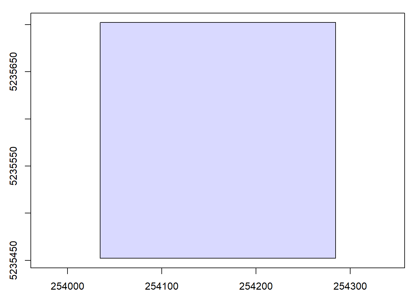
#> Chunk 1 of 4 (25%): state ✓
#>

Chunk 2 of 4 (50%): state ✓
#>

Chunk 3 of 4 (75%): state ✓
#>

Chunk 4 of 4 (100%): state ✓
#>
# Read catalog of plots
ctg_plots <- readLAScatalog(tempdir())

# Set independent files option
opt_independent_files(ctg_plots) <- TRUE
opt_output_files(ctg_plots) <- paste0(tempdir(),"/{XCENTER}_{XCENTER}")

# Generate plot-level terrain models
rasterize_terrain(las = ctg_plots, res = 1, algorithm = tin())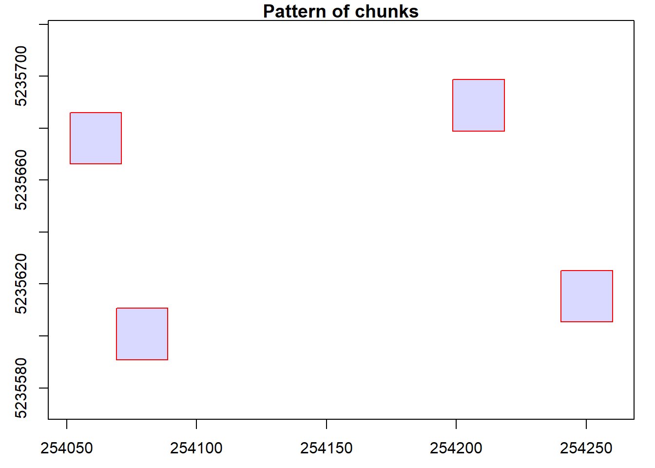
#> Chunk 1 of 4 (25%): state ✓
#>

Chunk 2 of 4 (50%): state ✓
#>

Chunk 3 of 4 (75%): state ✓
#>

Chunk 4 of 4 (100%): state ✓
#>

#> class       : SpatRaster
#> size        : 204, 208, 1  (nrow, ncol, nlyr)
#> resolution  : 1, 1  (x, y)
#> extent      : 254035, 254243, 5235460, 5235664  (xmin, xmax, ymin, ymax)
#> coord. ref. : NAD83(CSRS) / MTM zone 7 (EPSG:2949)
#> source      : rasterize_terrain.vrt
#> name        :          Z
#> min value   :  767.23999
#> max value   : 780.429993
# Check files
path <- paste0(tempdir())
file_list <- list.files(path, full.names = TRUE)
file <- file_list[grep("\\.tif$", file_list)][[1]]
# plot dtm
plot(terra::rast(file))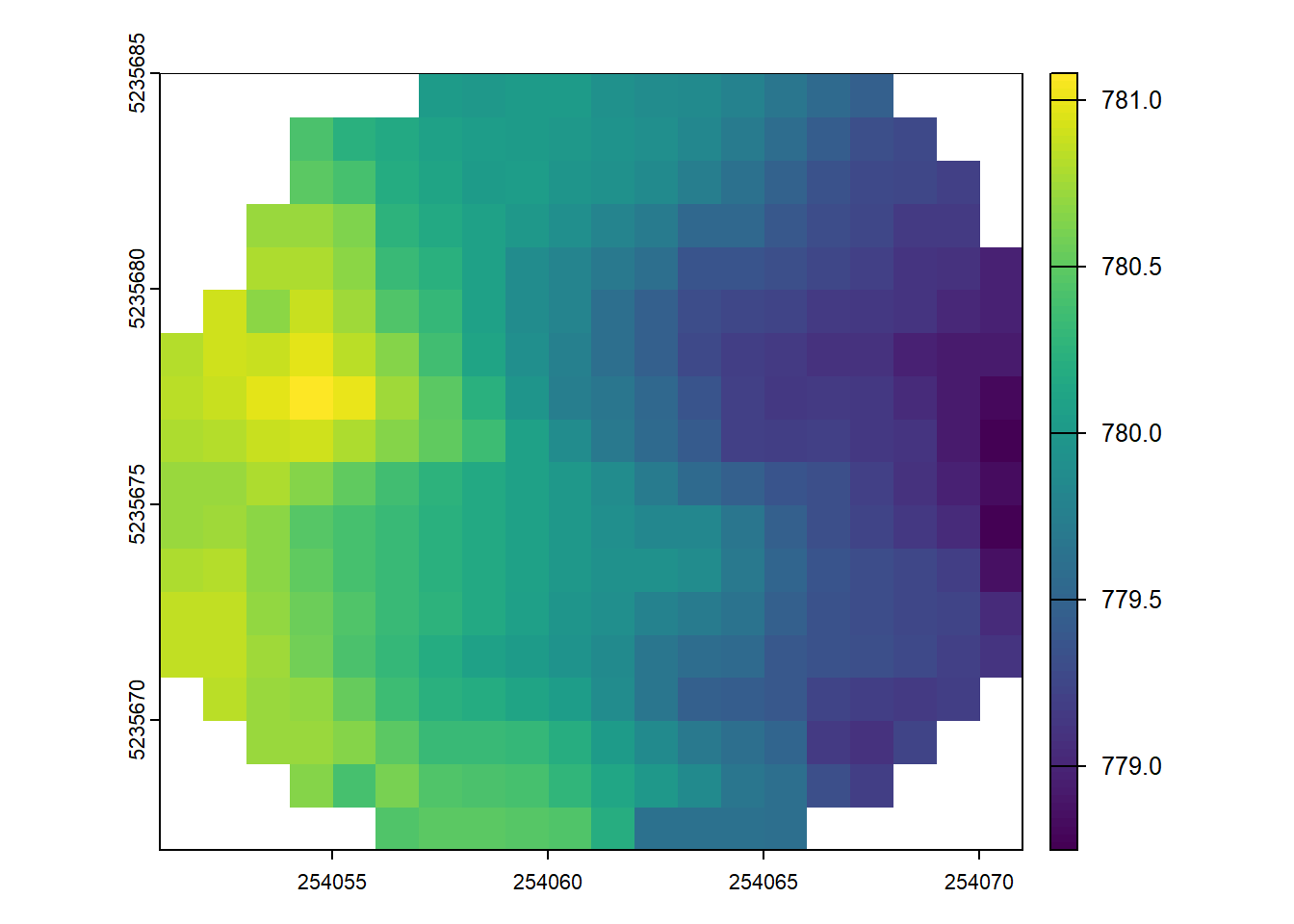
Conclusion
This concludes our tutorial on selecting simple geometries and extracting complex geometries from geopackage files (or shapefiles etc…) using the lidR package in R.