This code demonstrates individual tree segmentation (ITS) using lidar data. It covers CHM-based and point cloud-based methods for tree detection and segmentation. The code also shows how to extract metrics at the tree level and visualize them.
Environment
# Clear environmentrm(list =ls(globalenv()))# *Ensure 'concaveman' is installed for tree segmentation*if (!requireNamespace("concaveman", quietly =TRUE)) {install.packages("concaveman", repos ="https://cloud.r-project.org")}# Load all required packageslibrary(concaveman)library(lidR)library(sf)library(terra)# Read in LiDAR file and set some color paletteslas <-readLAS("data/fm_norm.laz")
col <-height.colors(50)col1 <-pastel.colors(900)
CHM based methods
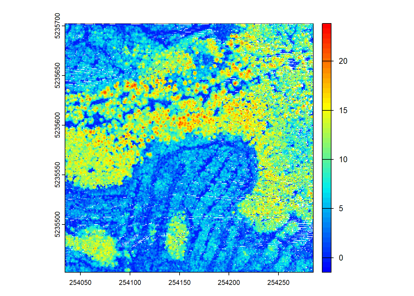
We start by creating a Canopy Height Model (CHM) from the lidar data. The rasterize_canopy() function generates the CHM using a specified resolution (res) and a chosen algorithm, here p2r(0.15), to compute the percentiles.
# Generate CHMchm <-rasterize_canopy(las = las, res =0.5, algorithm =p2r(0.15))plot(chm, col = col)
After building the CHM, we visualize it using a color palette (col).
Optionally smooth the CHM
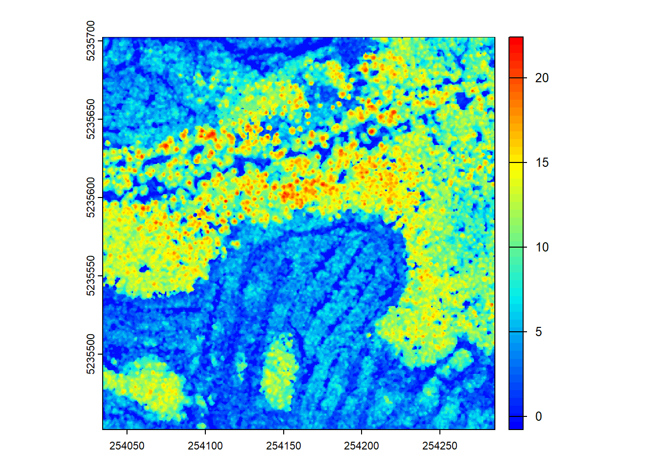
Optionally, we can smooth the CHM using a kernel to remove small-scale variations and enhance larger features like tree canopies.
# Generate kernel and smooth chmkernel <-matrix(1, 3, 3)schm <- terra::focal(x = chm, w = kernel, fun = median, na.rm =TRUE)plot(schm, col = col)
Here, we smooth the CHM using a median filter with a 3x3 kernel. The smoothed CHM (schm) is visualized using a color palette to represent height values.
Tree detection
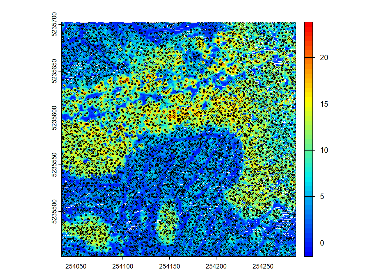
Next, we detect tree tops using the smoothed CHM. The locate_trees() function identifies tree tops based on local maxima.
# Detect treesttops <-locate_trees(las = schm, algorithm =lmf(ws =2.5))ttops#> Simple feature collection with 4694 features and 2 fields#> Attribute-geometry relationships: constant (2)#> Geometry type: POINT#> Dimension: XYZ#> Bounding box: xmin: 254034.8 ymin: 5235452 xmax: 254284.8 ymax: 5235702#> z_range: zmin: 2 zmax: 22.39#> Projected CRS: NAD83(CSRS) / MTM zone 7#> First 10 features:#> treeID Z geometry#> 1 1 4.960 POINT Z (254113.8 5235702 4...#> 2 2 4.350 POINT Z (254130.2 5235702 4...#> 3 3 7.000 POINT Z (254134.8 5235702 7)#> 4 4 5.550 POINT Z (254137.2 5235702 5...#> 5 5 5.000 POINT Z (254143.8 5235702 5)#> 6 6 6.250 POINT Z (254147.2 5235702 6...#> 7 7 4.620 POINT Z (254154.8 5235702 4...#> 8 8 4.450 POINT Z (254158.8 5235702 4...#> 9 9 3.125 POINT Z (254163.8 5235702 3...#> 10 10 6.560 POINT Z (254169.8 5235702 6...plot(chm, col = col)plot(ttops, col ="black", add =TRUE, cex =0.5)
The detected tree tops (ttops) are plotted on top of the CHM (chm) to visualize their positions.
Segmentation
Now, we perform tree segmentation using the detected tree tops. The segment_trees() function segments the trees in the lidar point cloud based on the previously detected tree tops.
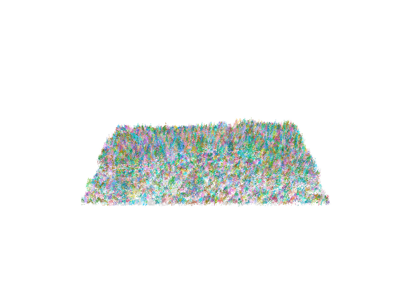
# Segment trees using dalpontelas <-segment_trees(las = las, algorithm =dalponte2016(chm = schm, treetops = ttops))
# Count number of trees detected and segmentedlength(unique(las$treeID) |>na.omit())#> [1] 4602tree_ids <-unique(las$treeID)
After segmentation, we count the number of trees detected and visualize all the trees in the point cloud. We then select two trees (tree25 and tree100) and visualize them individually.
NoteVariability and testing
Forests are highly variable! This means that some algorithms and parameters will work better than others depending on the data you have. Play around with algorithms and see which works best for your data.
Working with rasters
The lidR package is designed for point clouds, but some functions can be applied to raster data as well. Here, we show how to extract trees from the CHM without using the point cloud directly.
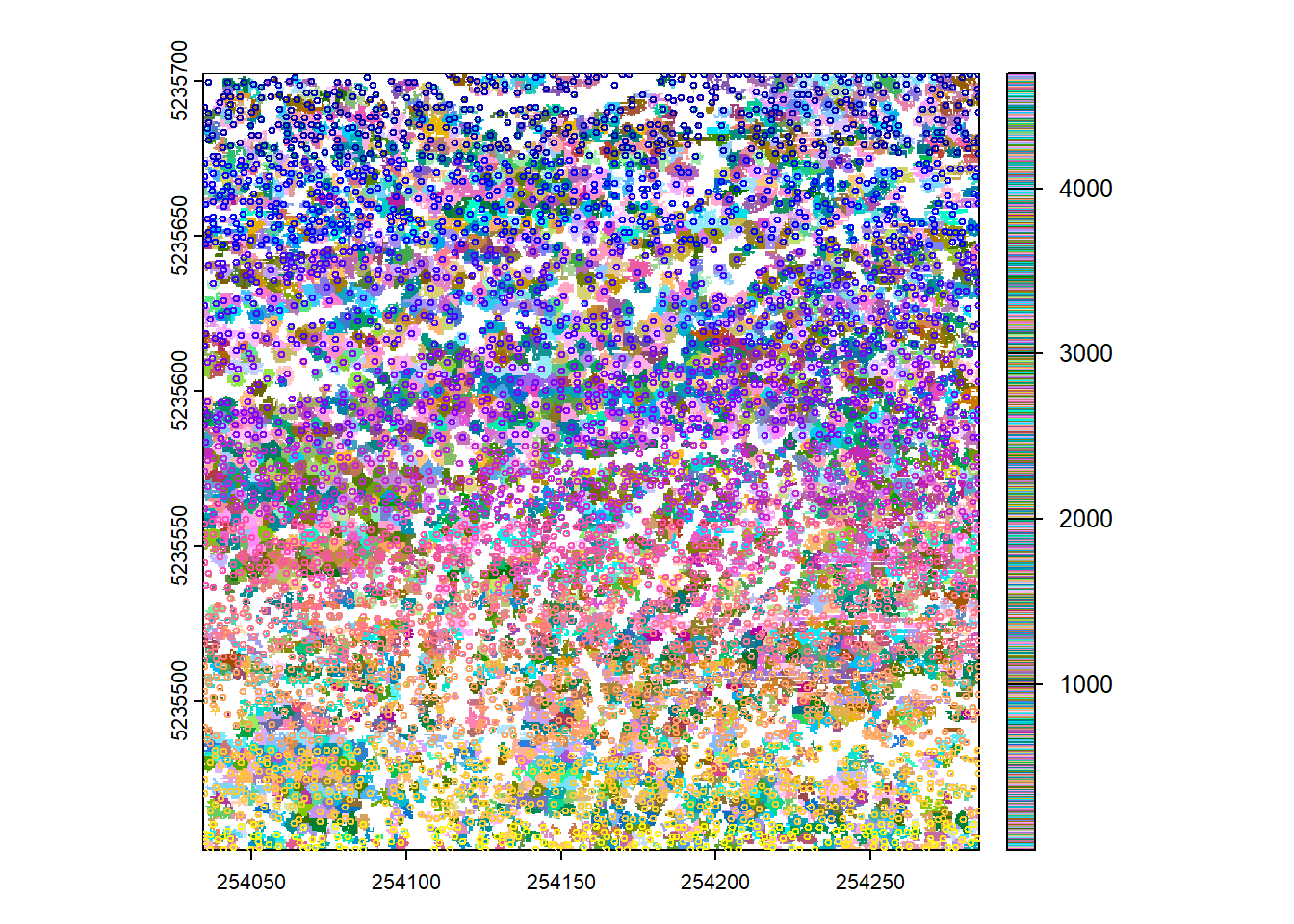
# Generate rasterized delineationtrees <-dalponte2016(chm = chm, treetops = ttops)() # Notice the parenthesis at the endtrees#> class : SpatRaster#> size : 501, 501, 1 (nrow, ncol, nlyr)#> resolution : 0.5, 0.5 (x, y)#> extent : 254034.5, 254285, 5235452, 5235702 (xmin, xmax, ymin, ymax)#> coord. ref. : NAD83(CSRS) / MTM zone 7 (EPSG:2949)#> source(s) : memory#> name : Z#> min value : 1#> max value : 4694plot(trees, col = col1)plot(ttops, add =TRUE, cex =0.5)#> Warning in plot.sf(ttops, add = TRUE, cex = 0.5): ignoring all but the first#> attribute
We create tree objects (trees) using the dalponte2016 algorithm with the CHM and tree tops. The resulting objects are visualized alongside the detected tree tops.
Point-cloud based methods (no CHM)
In this section, we will explore tree detection and segmentation methods that do not require a CHM.
Tree detection
We begin with tree detection using the local maxima filtering (lmf) algorithm. This approach directly works with the lidar point cloud to detect tree tops.
We detect tree tops using the lmf algorithm and visualize them in 3D by adding the tree tops to the lidar plot.
Tree segmentation
Next, we perform tree segmentation using the li2012 algorithm, which directly processes on the lidar point cloud instead of the CHM.
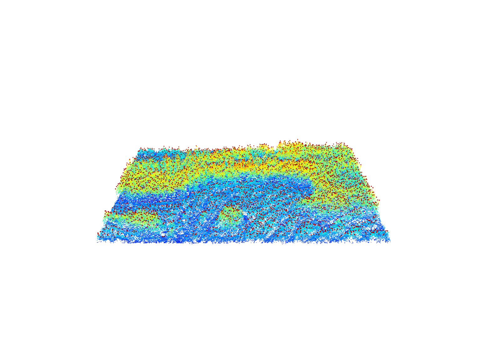
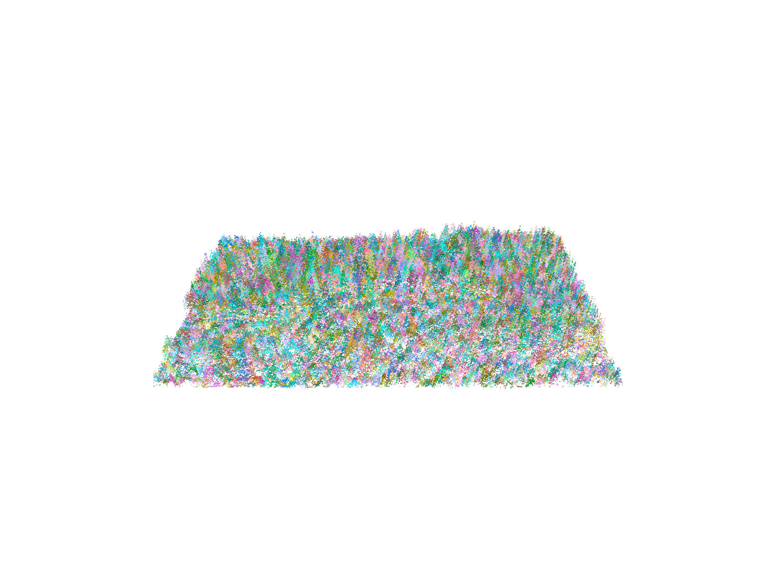
# Segment using lilas <-segment_trees(las = las, algorithm =li2012())
plot(las, color ="treeID")# This algorithm does not seem pertinent for this dataset.
The li2012 algorithm segments the trees in the lidar point cloud based on local neighborhood information. However, it may not be optimal for this specific dataset.
Extraction of metrics
We will extract various metrics from the tree segmentation results.
Using crown_metrics()
The crown_metrics() function extracts metrics from the segmented trees using a user-defined function. We use the length of the Z coordinate to obtain the tree height as an example.
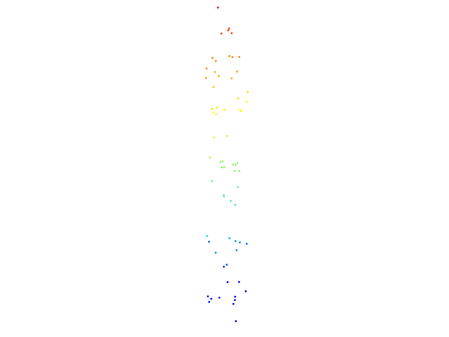
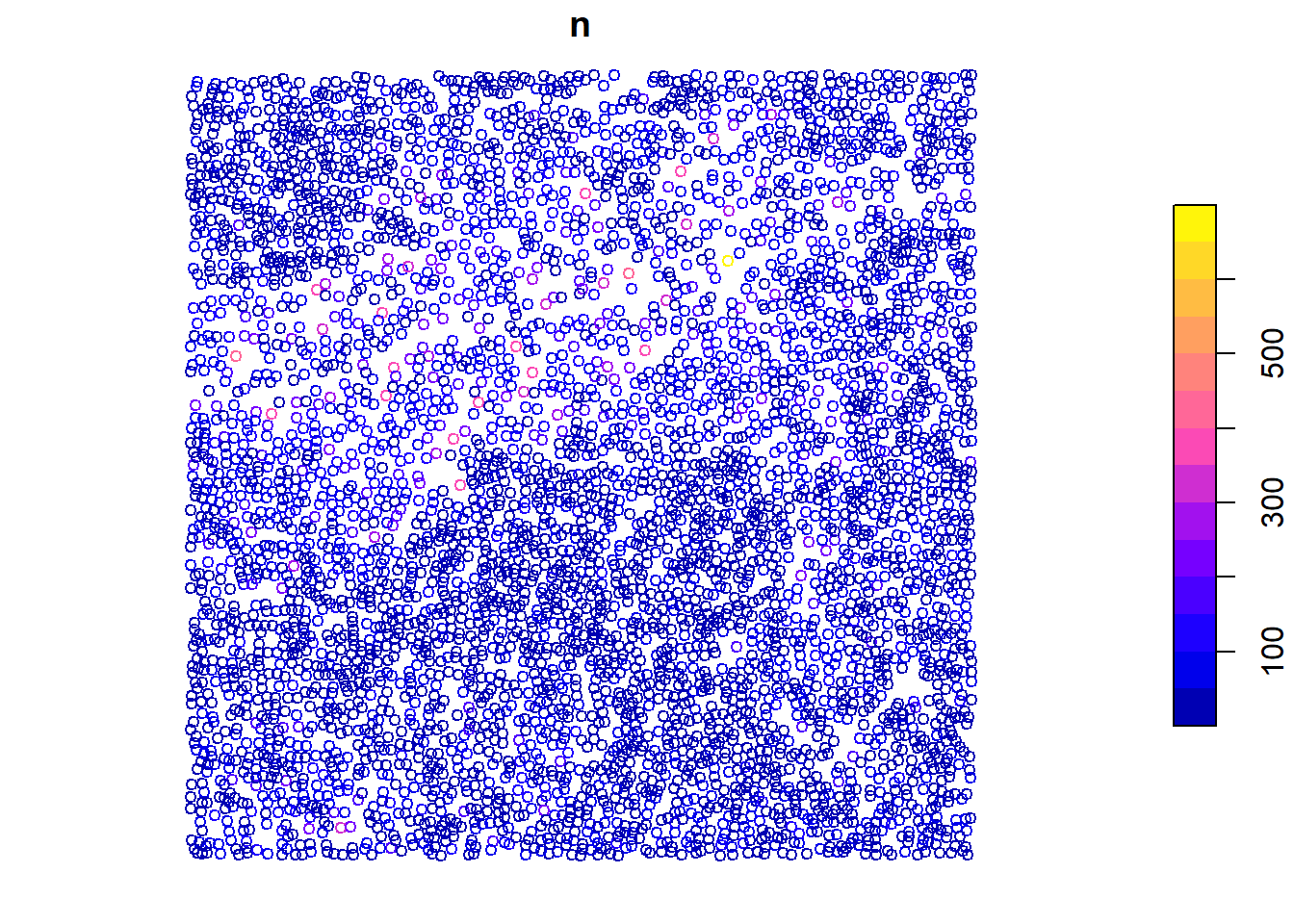
# Generate metrics for each delineated crownmetrics <-crown_metrics(las = las, func =~list(n =length(Z)))metrics#> Simple feature collection with 4895 features and 2 fields#> Geometry type: POINT#> Dimension: XYZ#> Bounding box: xmin: 254034.6 ymin: 5235452 xmax: 254284.6 ymax: 5235702#> z_range: zmin: 2.03 zmax: 23.83#> Projected CRS: NAD83(CSRS) / MTM zone 7#> First 10 features:#> treeID n geometry#> 1 1 248 POINT Z (254097.6 5235640 2...#> 2 2 137 POINT Z (254154.3 5235608 2...#> 3 3 146 POINT Z (254103.9 5235629 2...#> 4 4 100 POINT Z (254113.3 5235598 2...#> 5 5 137 POINT Z (254158.8 5235611 2...#> 6 6 113 POINT Z (254101.9 5235579 2...#> 7 7 235 POINT Z (254175.1 5235608 2...#> 8 8 166 POINT Z (254120.4 5235603 2...#> 9 9 99 POINT Z (254150.3 5235607 2...#> 10 10 157 POINT Z (254139.6 5235639 2...plot(metrics["n"], cex =0.8)
We calculate the number of points (n) in each tree crown using a user-defined function, and then visualize the results.
Applying user-defined functions
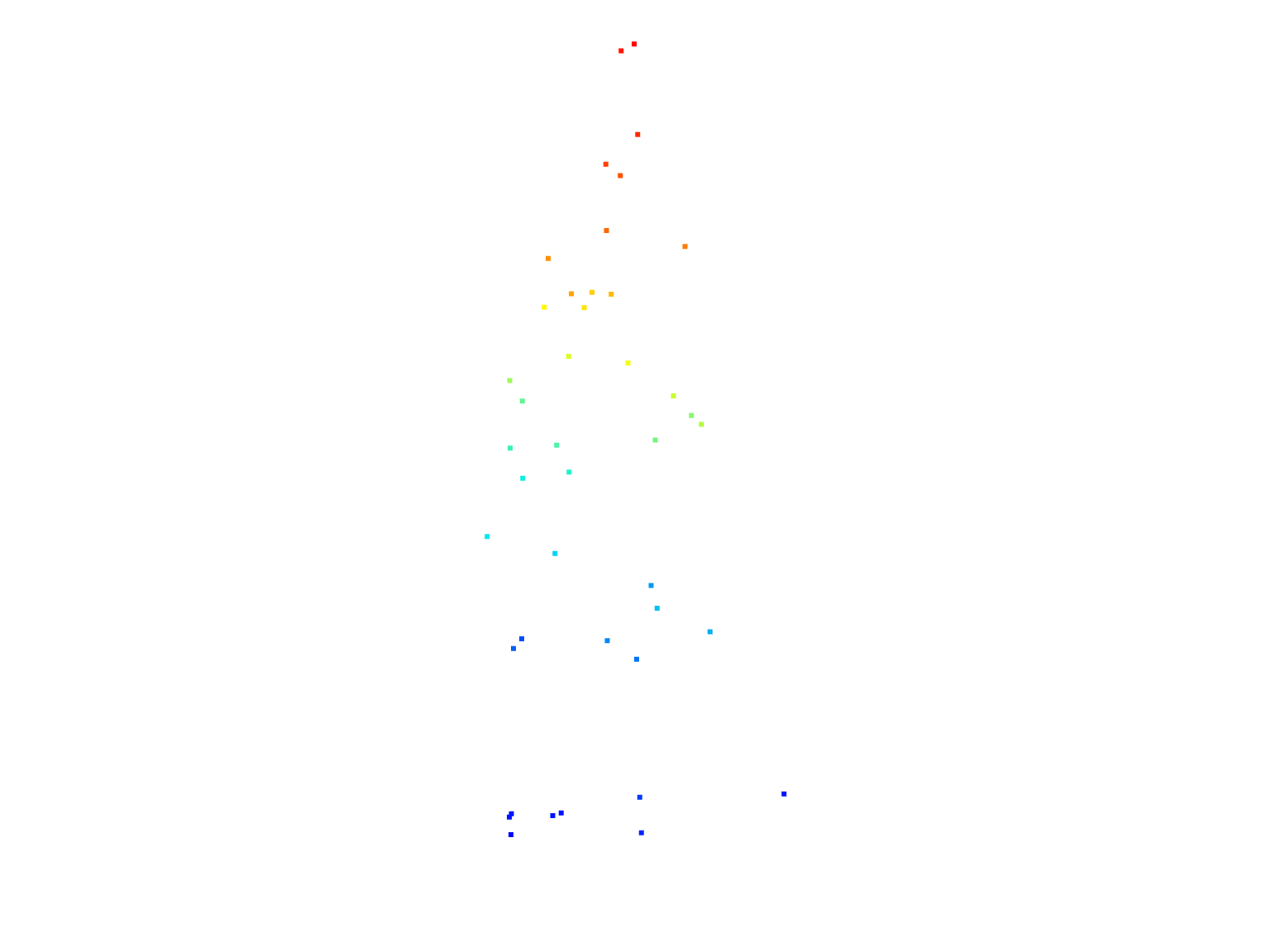
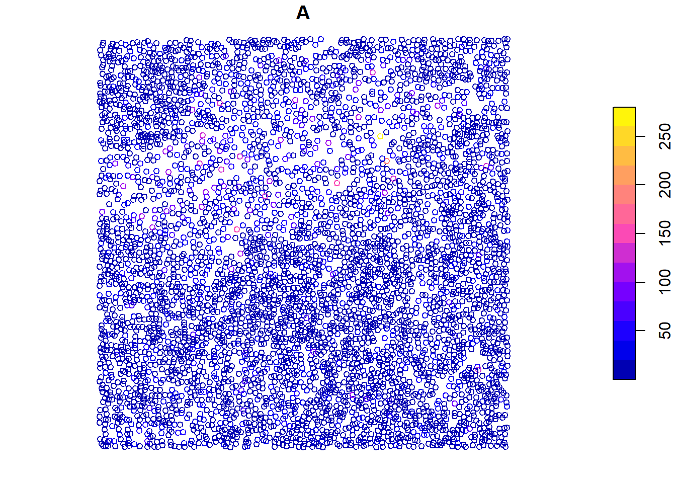
We can map any user-defined function at the tree level using the crown_metrics() function, just like pixel_metrics(). Here, we calculate the convex hull area of each tree using a custom function f() and then visualize the results.
# User defined function for area calculationf <-function(x, y) {# Get xy for tree coords <-cbind(x, y)# Convex hull ch <-chull(coords)# Close coordinates ch <-c(ch, ch[1]) ch_coords <- coords[ch, ]# Generate polygon p <- sf::st_polygon(list(ch_coords))#calculate area area <- sf::st_area(p)return(list(A = area))}# Apply user-defined functionmetrics <-crown_metrics(las = las, func =~f(X, Y))metrics#> Simple feature collection with 4895 features and 2 fields#> Geometry type: POINT#> Dimension: XYZ#> Bounding box: xmin: 254034.6 ymin: 5235452 xmax: 254284.6 ymax: 5235702#> z_range: zmin: 2.03 zmax: 23.83#> Projected CRS: NAD83(CSRS) / MTM zone 7#> First 10 features:#> treeID A geometry#> 1 1 82.43385 POINT Z (254097.6 5235640 2...#> 2 2 24.97670 POINT Z (254154.3 5235608 2...#> 3 3 25.50170 POINT Z (254103.9 5235629 2...#> 4 4 15.56400 POINT Z (254113.3 5235598 2...#> 5 5 20.40200 POINT Z (254158.8 5235611 2...#> 6 6 21.57695 POINT Z (254101.9 5235579 2...#> 7 7 40.53795 POINT Z (254175.1 5235608 2...#> 8 8 26.37255 POINT Z (254120.4 5235603 2...#> 9 9 17.88695 POINT Z (254150.3 5235607 2...#> 10 10 31.20635 POINT Z (254139.6 5235639 2...plot(metrics["A"], cex =0.8)
Tip3rd party metric packages
Remember that you can use 3rd party packages like lidRmetrics for crown metrics too!
Using pre-defined metrics
Some metrics are already recorded, and we can directly calculate them at the tree level using crown_metrics().
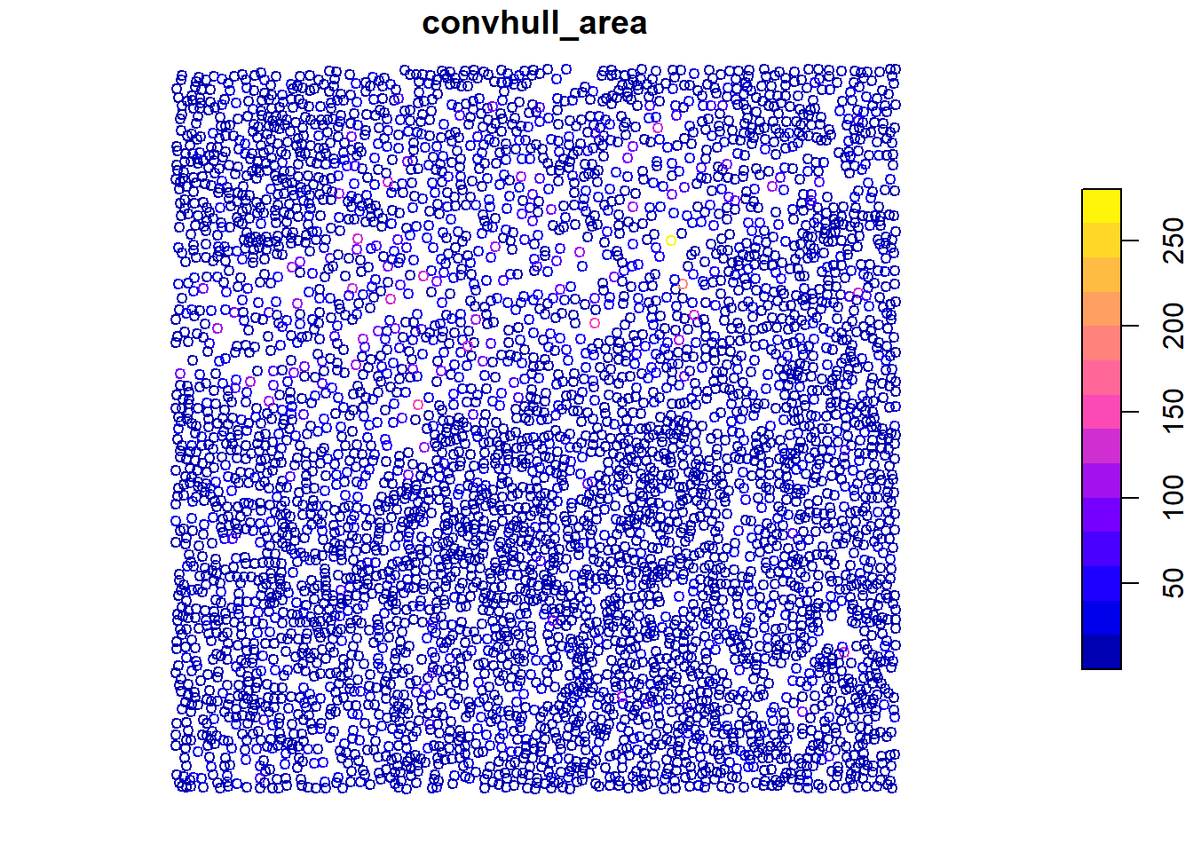
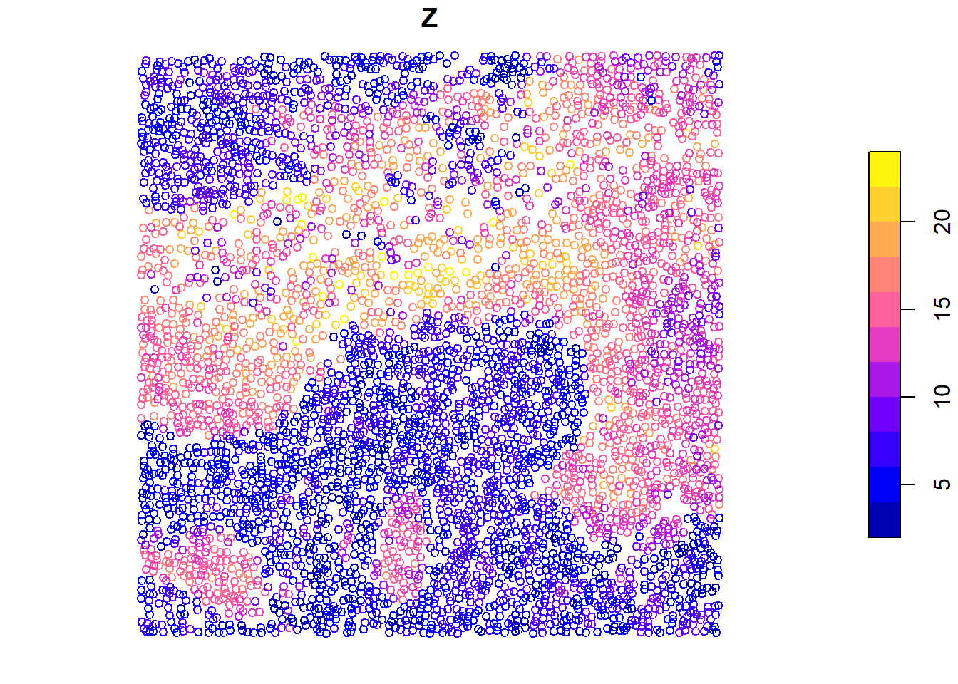
metrics <-crown_metrics(las = las, func = .stdtreemetrics)metrics#> Simple feature collection with 4895 features and 4 fields#> Geometry type: POINT#> Dimension: XYZ#> Bounding box: xmin: 254034.6 ymin: 5235452 xmax: 254284.6 ymax: 5235702#> z_range: zmin: 2.03 zmax: 23.83#> Projected CRS: NAD83(CSRS) / MTM zone 7#> First 10 features:#> treeID Z npoints convhull_area geometry#> 1 1 23.83 248 82.434 POINT Z (254097.6 5235640 2...#> 2 2 23.57 137 24.977 POINT Z (254154.3 5235608 2...#> 3 3 23.45 146 25.502 POINT Z (254103.9 5235629 2...#> 4 4 23.29 100 15.564 POINT Z (254113.3 5235598 2...#> 5 5 22.80 137 20.402 POINT Z (254158.8 5235611 2...#> 6 6 22.79 113 21.577 POINT Z (254101.9 5235579 2...#> 7 7 22.79 235 40.538 POINT Z (254175.1 5235608 2...#> 8 8 22.72 166 26.373 POINT Z (254120.4 5235603 2...#> 9 9 22.66 99 17.887 POINT Z (254150.3 5235607 2...#> 10 10 22.45 157 31.206 POINT Z (254139.6 5235639 2...# Visualize individual metricsplot(x = metrics["convhull_area"], cex =0.8)
plot(x = metrics["Z"], cex =0.8)
We calculate tree-level metrics using .stdtreemetrics and visualize individual metrics like convex hull area and height.
Delineating crowns
The crown_metrics() function segments trees and extracts metrics at the crown level.
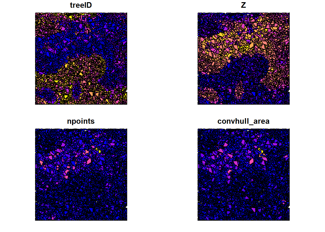
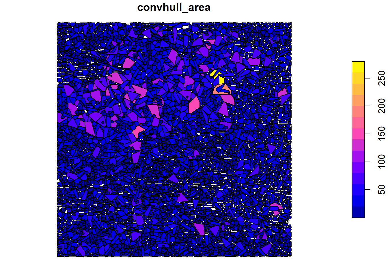
# Visualize individual metrics based on valuesplot(x = cvx_hulls["convhull_area"])
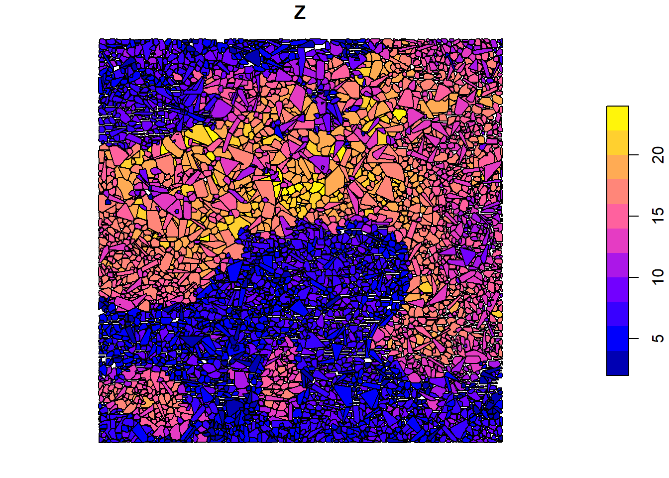
plot(x = cvx_hulls["Z"])
We use crown_metrics() with .stdtreemetrics to segment trees and extract metrics based on crown delineation.
ITD using LAScatalog
In this section, we explore Individual Tree Detection (ITD) using the LAScatalog. We first configure catalog options for ITD.
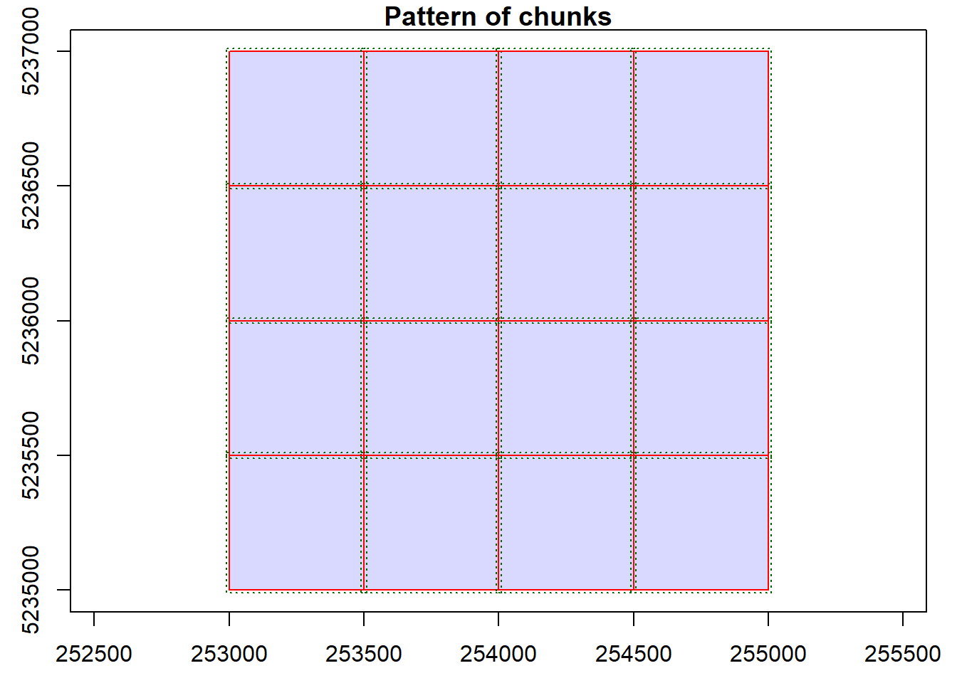
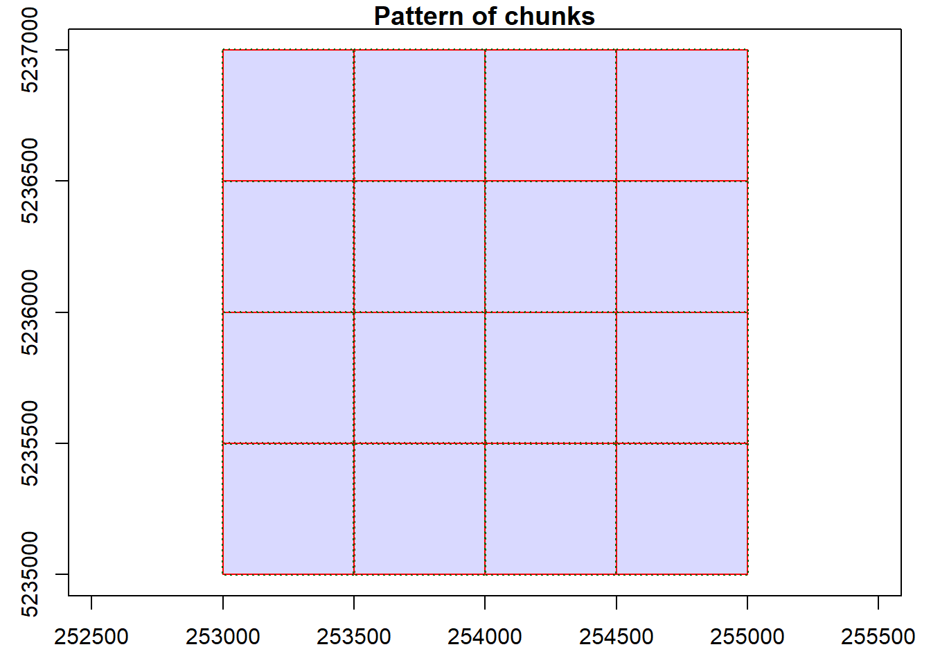
# Load catalogctg <-catalog('data/ctg_norm')# Set catalog optionsopt_filter(ctg) <-"-drop_z_below 0 -drop_z_above 50"opt_select(ctg) <-"xyz"opt_chunk_size(ctg) <-500opt_chunk_buffer(ctg) <-10opt_progress(ctg) <-TRUE# Explicitly tell R to use the is.empty function from the lidR package - avoid terra erroris.empty <- lidR::is.empty# Detect treetops and plotttops <-locate_trees(las = ctg, algorithm =lmf(ws =3, hmin =10))
#> Chunk 1 of 16 (6.2%): state ✓
#>
Chunk 2 of 16 (12.5%): state ✓
#>
Chunk 3 of 16 (18.8%): state ✓
#>
Chunk 4 of 16 (25%): state ✓
#>
Chunk 5 of 16 (31.2%): state ✓
#>
Chunk 6 of 16 (37.5%): state ✓
#>
Chunk 7 of 16 (43.8%): state ✓
#>
Chunk 8 of 16 (50%): state ✓
#>
Chunk 9 of 16 (56.2%): state ✓
#>
Chunk 10 of 16 (62.5%): state ✓
#>
Chunk 11 of 16 (68.8%): state ✓
#>
Chunk 12 of 16 (75%): state ✓
#>
Chunk 13 of 16 (81.2%): state ✓
#>
Chunk 14 of 16 (87.5%): state ✓
#>
Chunk 15 of 16 (93.8%): state ✓
#>
Chunk 16 of 16 (100%): state ✓
#>
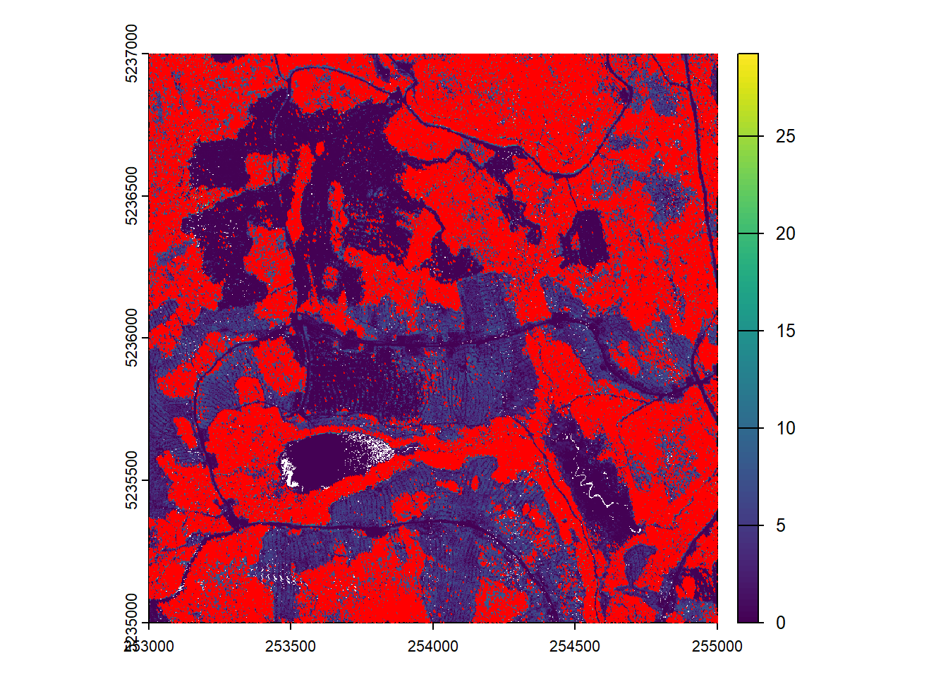
chm <- rasterize_canopy(ctg, algorithm = p2r(), res = 1)
#> Chunk 1 of 16 (6.2%): state ✓
#>

Chunk 2 of 16 (12.5%): state ✓
#>

Chunk 3 of 16 (18.8%): state ✓
#>

Chunk 4 of 16 (25%): state ✓
#>

Chunk 5 of 16 (31.2%): state ✓
#>

Chunk 6 of 16 (37.5%): state ✓
#>

Chunk 7 of 16 (43.8%): state ✓
#>

Chunk 8 of 16 (50%): state ✓
#>

Chunk 9 of 16 (56.2%): state ✓
#>

Chunk 10 of 16 (62.5%): state ✓
#>

Chunk 11 of 16 (68.8%): state ✓
#>

Chunk 12 of 16 (75%): state ✓
#>

Chunk 13 of 16 (81.2%): state ✓
#>

Chunk 14 of 16 (87.5%): state ✓
#>

Chunk 15 of 16 (93.8%): state ✓
#>

Chunk 16 of 16 (100%): state ✓
#>

plot(chm)
plot(ttops, add = TRUE, cex = 0.1, col = "red")
Conclusion
This concludes the tutorial on various methods for tree detection, segmentation, and extraction of metrics using the lidR package in R.