library(lidR) # For processing lidar data
library(dplyr) # For data manipulation
library(sf) # For manipulation of vector datasets
library(terra) # For raster manipulation
library(siplab) # For calculating competition metrics

las <- readLAS('extdata/thin_plot_dec.laz')Lidar Competition Metrics Workflow
Quantifying Tree-level Competition Metrics and Crown Volume with Drone Lidar Data - Irwin et al. 2024
Overview
In this document we will provide a brief overview of the processing steps required to go from a raw point cloud to a individual tree competition metric layer. This workflow is based on the methods outlined in Irwin et al. 2024 and is designed to be used with the R programming language.
1 - Normalized LAS point cloud
2 - Tree detection (lidR)
3 - Tree segmentation
4 - Computation of crown volume
5 - Computation of competition indices
Tree Detection and Segmentation
In this snippet we will start with a normalized lidar point cloud collected over a coniferous managed forest stand. In this stand managers have expressed desire to perform thinning but require a spatially explicit layer describing the competitive distribution of trees to prioritize their approach. Using this layer they can target areas or even trees with relatively high competition metrics as priority for thinning.
First we will detect and segment tree crowns, there are many methods to achieve this and they should be selected based on the objectives, forest type, and avaliable compute power (more details: lidRbook/itd-its). In this study we applied a modified marker-based watershed approach. Thanks to the distinct conical shape and distribution of the trees in these conifer dominated stands, this approach worked well for detecting and segmenting dominant and co-dominant trees that are the target for commercial thinning.
We will start by loading relevant packages and an example point cloud from the DJI L1 lidar dataset; a subset of the drone laser scanning data clipped from the Irwin et al. 2024 coverage. See the manuscript for details on acquisition parameters.
- To speed up computation in this tutorial, the point cloud has been thinned from the original density (~1200 pts/m2) using a 25 cm voxel retaining 1 random point for each, resulting in a final point density of (173 points/m2).
Download the point cloud here (8.05 mb)
First we will generate a canopy height model, smooth it, detect tree tops, and finally segment tree crowns.
Canopy Height Model Generation
# Generate 0.1m Canopy Height Model (CHM) with lidR
chm <- lidR::rasterize_canopy(las, res = 0.1, p2r(subcircle = 0.075))

# Gaussian smoothing function
fgauss <- function(sigma, n = ws) {
    m <- matrix(ncol = n, nrow = n)
    col <- rep(1:n, n)
    row <- rep(1:n, each = n)
    x <- col - ceiling(n/2)
    y <- row - ceiling(n/2)
    m[cbind(row, col)] <- 1/(2 * pi * sigma^2) * exp     (-(x^2 + y^2)/(2 * sigma^2))
    m/sum(m)
  }

# Apply Gaussian smoothing with terra::focal
chm <- terra::focal(chm, w = fgauss(1, n = 5), na.rm = T)

# Plot smoothed CHM
plot(chm, col = viridis::viridis(50))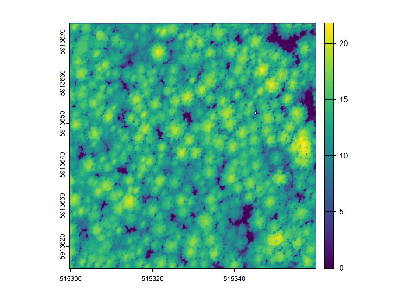
Tree top detection
# Locate local maxima (tree tops) across the smoothed CHM with 2m window
ttops <- locate_trees(chm, algorithm = lmf(ws = 2, shape = "circular"))

# Plot smoothed the CHM with detected local maxima overlaid
plot(chm, col = viridis::viridis(50))
plot(st_geometry(ttops), add = T, pch = 3, col = 'red', cex = 0.5)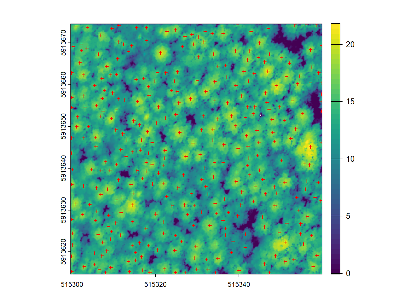
Tree crown segmentation
Functions
Watershed Segmentation
# Base watershed segmentation (requires EBimage)
mcwatershed <-function(chm, treetops, th_tree = 2, tree_id = "treeID")
{
  f = function(bbox)
  {
    if (!missing(bbox)) chm <- terra::crop(chm, bbox)

    # Convert the CHM to a matrix
    Canopy <- terra::as.matrix(chm, wide = TRUE)
    mask   <- Canopy < th_tree | is.na(Canopy)
    Canopy[mask] <- 0

    cells <- terra::cellFromXY(chm, sf::st_coordinates(treetops)[, c(1, 2)])
    ids <- dplyr::pull(treetops, tree_id)

    seeds = chm
    seeds[] = 0L
    seeds[cells] = ids
    treetops = terra::as.matrix(seeds, wide = TRUE)

    Canopy <- Canopy/max(Canopy)
    Canopy <- imager::as.cimg(Canopy)
    treetops  <- imager::as.cimg(treetops)
    Crowns <- imager::watershed(treetops, Canopy)
    Crowns <- Crowns[,,1,1]

    Crowns[mask] <- NA_integer_
    out <- terra::setValues(chm, Crowns)

    return(out)
  }

  f <- lidR::plugin_its(f, raster_based = TRUE)
  return(f)
}
Modified Height Limited approach
This approach limits watershed crown segmentation using a canopy height pixel threshold parameter that is set as a multiple of tree height. In this sense a 10 m tall tree crown could not contain CHM pixels less than 7 m in height. This approach is very useful in dense closed canopy stands to reduce over-segmentation and constraint watershed results.
# Height limited watershed segmentation function
crown_mask <- function(chunk, ttops = NULL, chm_res = 0.25, crown_height_threshold = 0.7, hmin = 2){

  # Check that 'chunk' is not missing or NULL
  if (is.null(chunk) || missing(chunk)) {
    stop("Error: 'chunk' argument must be specified.")
  }

  # Check if input is a SpatRaster object
  if("SpatRaster" == class(chunk)){
    chm <- chunk
    chm_res <- terra::res(chm)[1]
    print('Input is SpatRaster (Presuming CHM) proceeding with crown segmentation')
  } else{
    # Check if input is a las file
    if("LAS" %in% class(chunk)){
      las <- chunk
      print('Input is las file proceeding with crown segmentation')
    }
    else{
      # Check if input is a las catalog chunk
      las <- lidR::readLAS(chunk)
      if (lidR::is.empty(las)) {
        return(NULL)
      }
      print('Input is catalog tile proceeding with crown segmentation')
    }

    # Generate canopy height
    chm <- lidR::rasterize_canopy(las, res = chm_res , lidR::p2r(na.fill = lidR::knnidw()))
  }

  # Initial crown segmentation
  crowns <- mcwatershed(chm, ttops, th_tree = hmin, tree_id = 'treeID')()
  # Replace crown IDs with maximum canopy height within crown
  crowns_max <- terra::classify(x = crowns,
                                rcl = as.data.frame(terra::zonal(chm,
                                                                 crowns,
                                                                 fun = 'max')))
  # Make CHM mask raster where height is less than threshold percent
  chm_mask <- chm
  chm_mask[chm_mask < (crown_height_threshold * crowns_max)] = NA
  # Re-run segmentation on masked CHM
  crowns_masked <- mcwatershed(chm_mask, ttops, th_tree = hmin, tree_id = 'treeID')()

  return(crowns_masked)
}
Fill watershed segmentations and keep largest crown polygon for each tree
This function is used to clean up the holes in segmentations resulting from the height limited approach, and to take the resulting largest polygon that is assumed to be the tree crown.
# Keep and fill largest crown polygon for each tree
convert_multi_to_single_polygons <- function(polygons, fill_holes = TRUE){
tictoc::tic()
if(!"MULTIPOLYGON" %in% unique(sf::st_geometry_type(polygons))){
  print('ERROR: Input sf polygon df contained zero MUTLIPOLYGONS; conversion not neccessary')
  stop()
}
# Seperate out multipolygons
mp <- polygons %>% dplyr::filter(sf::st_geometry_type(polygons) == 'MULTIPOLYGON')
# Seperate out polygons
sp <- polygons %>% dplyr::filter(sf::st_geometry_type(polygons) == 'POLYGON')

largest_polygon <- function(x, Z) {
  # Turn multipolygon into vector of single polygons
  x <- sf::st_combine(x)
  x <- sf::st_cast(x, "POLYGON")
  # Calculate area of each single polygon
  areas <- sf::st_area(x)
  # Take largest polygon
  max_area_index <- which.max(areas)
  # Re-add the attribute column
  largest <- x[max_area_index] %>% sf::st_as_sf(crs = sf::st_crs(x))
  # Re-name geometry column
  sf::st_geometry(largest) <- 'geometry'
  largest <- cbind(largest, Z) %>% dplyr::relocate(geometry, .after = tidyselect::last_col())
  if(fill_holes){
  # Fill any holes in the resulting polygon
  largest <- nngeo::st_remove_holes(largest)
  }
  return(largest)
}

# Go through multipolygons and apply largest_polygon function
# Empty list for fixed polygons
p_polygons <- list()
# Progress bar
pb <- progress::progress_bar$new(total = nrow(mp))
print('Taking largest polygon of each MULTIPOLYGON crown')
for (i in 1:nrow(mp)) {
  p_polygons[[i]] <- largest_polygon(sf::st_geometry(mp[i,]), Z = sf::st_drop_geometry(mp[i,]))
  pb$tick()
}
# Bind list of corrected polygons
print(glue::glue('Binding together {length(p_polygons)} cleaned polygons'))
p_polygons <- do.call(rbind, p_polygons)
sf::st_crs(p_polygons) <- sf::st_crs(polygons)
if(fill_holes == TRUE & nrow(sp) > 0){
# Fill holes in single polygon polygons
sp <- nngeo::st_remove_holes(sp)
}
# Re-join all polygons together
polygons <- rbind(sp, p_polygons)
print(glue::glue('Finished cleaning {nrow(polygons)} polygons'))
tictoc::toc()
return(polygons)
}
Calculate Tree Crown Volume
Apply treeID values from segmented tree crowns to point cloud
# Merge Crown ID with las point cloud
tree_las <- lidR::merge_spatial(las, crowns, attribute = 'treeID')
# Add treeID attribute to las
tree_las = add_lasattribute(tree_las, name = "treeID", desc = "ID of a tree")
# Filter out non tree points to speed up computation
tree_las <- filter_poi(tree_las, !is.na(treeID))
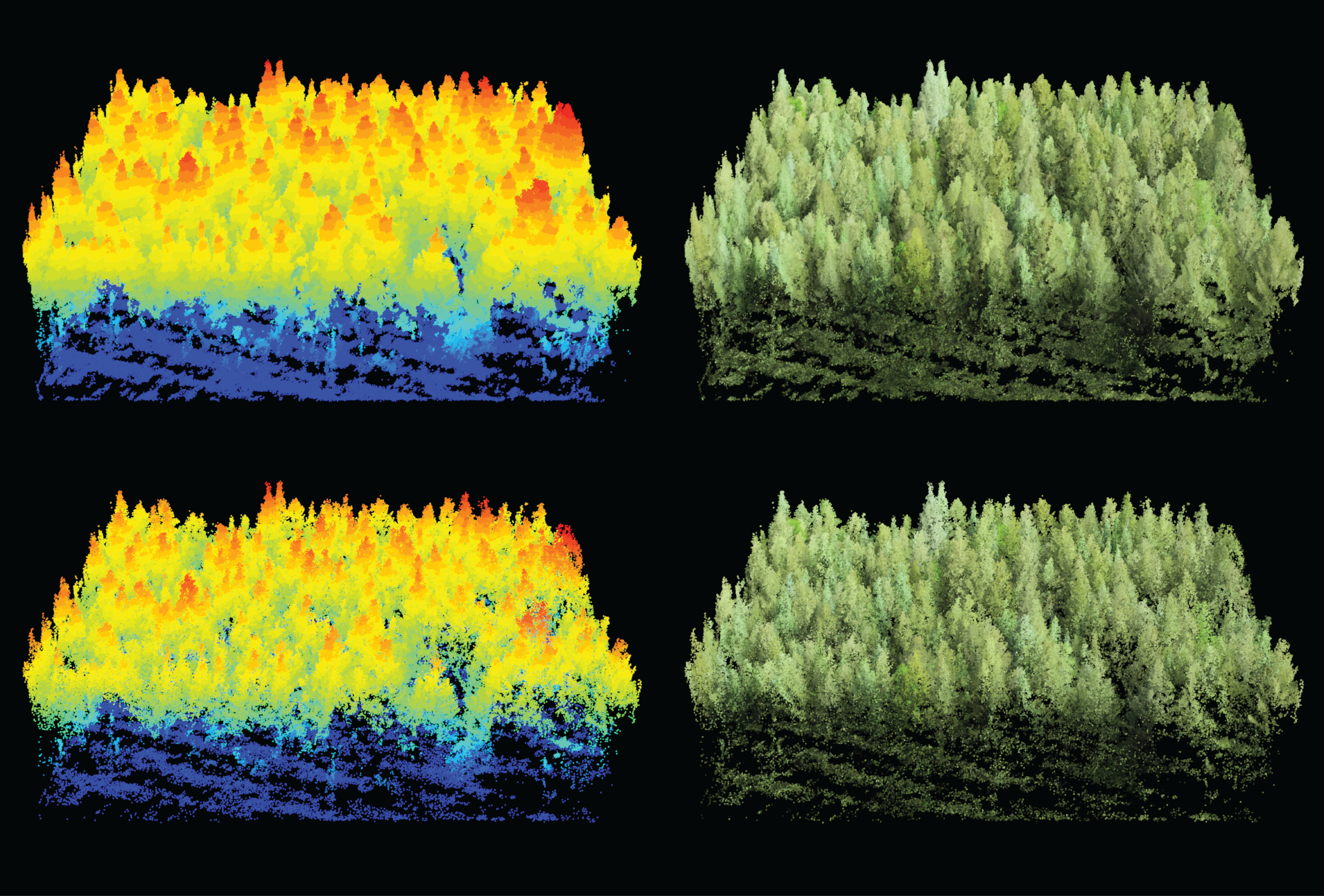
# Plot resulting point cloud coloured by treeID
plot(tree_las, color = 'treeID')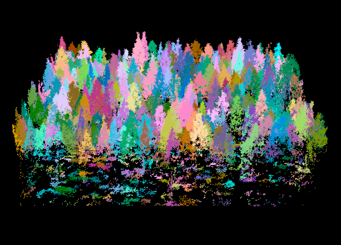
Generate 3D alphashape and calculate convex/concave hull (crown) volume for each tree
Functions
Compute alpha shape of a clipped lidar point cloud
This function takes an input individual tree lidar point cloud and computes and alpha shape using the alphashape3d package. To do so first any segmentation with less than 3 points are discarded (in practice there are few or none). Second the X, Y, and Z coordinates are normalized to be locally referenced. Next several metrics including the volume of the hull are calculated.
get_crown_attributes <- function(X,Y,Z){
  if (length(X) <= 3 || length(Y) <= 3 || length(Z) <= 3) {
    print('Cannot compute a 3D hull from 3 or fewer points')
    return(NULL)
  }
  # alphashadep3d
  a3d = cbind(X, Y, Z)
  # get treetop location
  top_x <- a3d[which.max(a3d[,3]),1]
  top_y <- a3d[which.max(a3d[,3]),2]
  # normalize X and Y
  a3d[,1] = a3d[,1] - mean(a3d[,1]) #center points around 0,0,0
  a3d[,2] = a3d[,2] - mean(a3d[,2]) #center points around 0,0,0
  alpha <- c(Inf, 1)
  ashape <- alphashape3d::ashape3d(x = a3d, alpha = alpha, pert = TRUE)

  # calculate crown metrics

  df <- data.frame(
    # Crown height metrics
    Zmax = max(Z),
    Zq999 = as.numeric(quantile(Z, 0.999)),
    Zq99 = as.numeric(quantile(Z, 0.990)),
    Z_mean = mean(Z),
    n_points = length(Z),
    # Crown size
    vol_convex = alphashape3d::volume_ashape3d(ashape, indexAlpha = 1),
    vol_concave = alphashape3d::volume_ashape3d(ashape, indexAlpha = 2),
    # Crown complexity
    CV_Z = sd(Z) / mean(Z),
    CRR = (mean(Z) - min(Z)) / (max(Z) - min(Z)),
    # Get tree top position
    X = top_x,
    Y = top_y)

  return(df)
}
The following is a lidR compatible function to compute these metrics across large areas.
To apply this across lidar tiles where treeIDs have been attributed to each relevant point we create this wrapper function that applies the above function across each tree ID.
get_alphashape_metrics <- function(chunk){

# Determine if input is chunk in a LAScatalog or a LAS object loaded in R
if ("LAS" %in% class(chunk)) {
    tree_las <- chunk
    print('Individual LAS object input into function')
} else{
tree_las <- lidR::readLAS(chunk)
}
# Check if input tile is empty
if (lidR::is.empty(tree_las)) return(NULL)

print(glue::glue('Beginning crown metric generation for chunk'))
# Remove duplicate points
tree_las <- lidR::filter_duplicates(tree_las)

# Organize data by treeID; remove trees with less than 4 points
obs <- tree_las@data %>%
  dplyr::filter(!is.na(treeID)) %>%
  dplyr::select(X, Y, Z, treeID) %>%
  dplyr::group_by(treeID) %>%
  dplyr::summarise(n = dplyr::n()) %>% dplyr::ungroup() %>% dplyr::filter(n <= 4)

if(nrow(obs) > 0){
print(glue::glue('{nrow(obs)} treeIDs had 4 or fewer points and were discarded'))
}

else{
  mets <- tree_las@data %>%
    dplyr::filter(!is.na(treeID)) %>%
    dplyr::filter(!treeID %in% obs$treeID) %>%
    dplyr::select(X,Y,Z,treeID) %>%
    dplyr::group_by(treeID) %>%
    # Apply get_crown_attributes function to each treeID
    dplyr::summarise(ashape_metrics = get_crown_attributes(X, Y, Z))
}

# Return data frame with treeID and crown metrics
mets <- cbind(mets$treeID, mets$ashape_metrics)
colnames(mets)[1] <- "treeID"

return(mets)

}
# Filter out points for one tree (example)
tree <- filter_poi(tree_las, treeID == 147)
# Calculate alphashape for tree
ashape <- get_crown_attributes(tree@data$X,
tree@data$Y,
tree@data$Z,
export_ashape = TRUE)
# Extract individual X,Y,Z points (for plotting)
a3d <- ashape[[3]]
# Extract alphashape object (for plotting)
ashape <- ashape[[2]]
# Plot Raw Point Cloud
plot(tree, bg = 'white', size = 6)
# Plot convex hull (alpha = Inf)
plot(ashape, indexAlpha = 1, transparency = 0.3, axes = TRUE)
rgl::points3d(a3d, color = 'black')
# Plot concave hull (alpha = 1)
plot(ashape, indexAlpha = 2, transparency = 0.4, axes = TRUE)
rgl::points3d(a3d, color = 'black')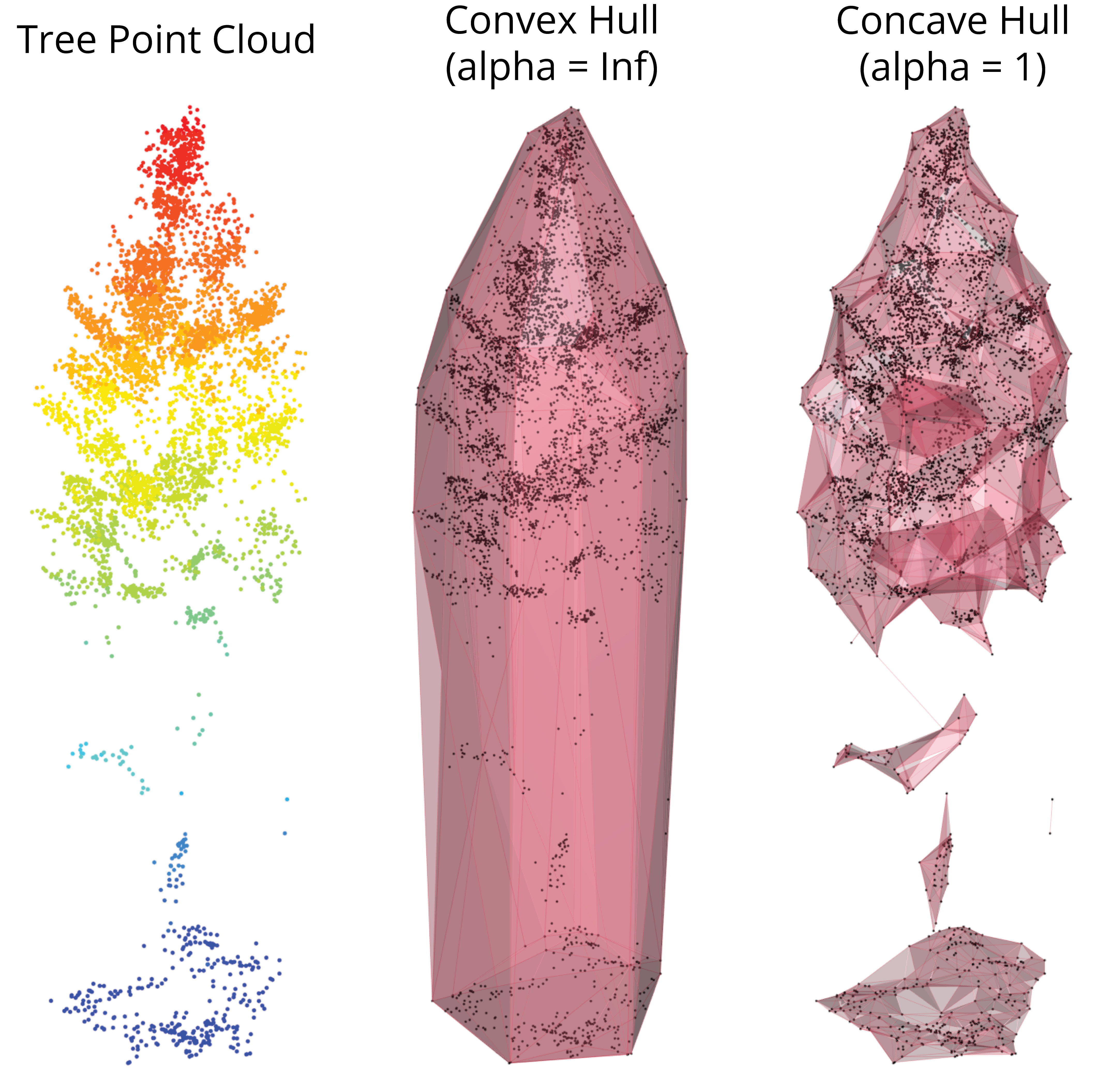
# Decimate density heavily to speed up alphashape computation in example
tree_las_dec <- decimate_points(tree_las, random_per_voxel(res = 0.5, n = 1))

# Calculate alphashape metrics across all trees in the LAS object
ashape_mets <- get_alphashape_metrics(tree_las)
[1] "Individual LAS object input into function"
Beginning crown metric generation for chunkCompute Competition Index
Calculate Competition Index based on Crown Volume Values

Functions
Calculate Heygi 1974 Pairwise Index with sf point objects (tree tops) This function will be used to take the detected tree tops from lidR (an sf point obect), convert them to a spatstat compatiable point pattern (ppp) object, and finally calculate the pairwise competition index using the siplap package. Read the paper on siplap here.
heygi_cindex <- function(ttops, comp_input = 'vol_convex', maxR = 6){
tictoc::tic()
# Reformat tree tops dataframe
trees_ppp <- ttops %>%
dplyr::mutate(X = X, Y = Y) %>%
as.data.frame() %>%
dplyr::select(c(X, Y, comp_input))
# Standardize column names
names(trees_ppp) <- c('X','Y','comp_value')
# Convert to spatstat ppp object
trees_ppp <- trees_ppp %>%
spatstat.geom::ppp(
x = .$X,
y = .$Y,
window = spatstat.geom::owin(range(.$X),
range(.$Y)),
marks = .$comp_value)
# Calculate heygi competition index for each tree (comp_input instead of dbh)
heygi <- trees_ppp %>%
siplab::pairwise(., maxR=maxR, kernel=siplab::powers_ker,
kerpar=list(pi=1, pj=1, pr=1, smark=1))
# Join new cindex with original ttops
trees_cindex <- heygi %>%
as.data.frame() %>% dplyr::select(x, y, cindex)
# Convert to sf object
ttops <- ttops %>% sf::st_as_sf(coords = c('X', 'Y'))
# Join cindex to tree tops sf object
trees_cindex <- dplyr::bind_cols(ttops, trees_cindex)
print(glue::glue('Calculated Heygi style competition for {nrow(trees_cindex)} trees assesing their {comp_input} within a {maxR}m radius'))
tictoc::toc()
return(trees_cindex)
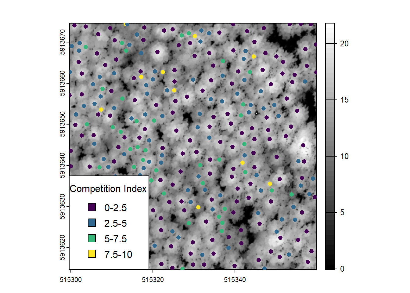
}Here we will take the above function and apply it to the tree tops attributed with the convex hull alpha shape volume from their associated point clouds. We will finish by plotting the result (filtered/binned to emphasize differences in index values).
# Calculate Heygi 1974 style Competition Index on tree tops attributed with crown volume values - remove one outliers one edge
heygi_6m <- heygi_cindex(ashape_mets, comp_input = 'vol_concave', maxR = 6) %>% filter(cindex < 10)
Calculated Heygi style competition for 335 trees assesing their vol_concave within a 6m radius
1.21 sec elapsed# Define the bins
breaks <- seq(0, 10, by = 2.5)
bin_labels <- paste(head(breaks, -1), tail(breaks, -1), sep = "-")
# Assign each cindex value to a bin
heygi_6m$cindex_bin <- cut(heygi_6m$cindex, breaks = breaks, labels = bin_labels, include.lowest = TRUE)
# Create a color mapping for the bins - ensuring one color per bin
c <- viridis::viridis(length(bin_labels))
# Map each bin to its color
bin_colors <- setNames(c, bin_labels)
cindex_bin_colors <- bin_colors[as.character(heygi_6m$cindex_bin)]
# Plot the CHM
plot(chm, col = colorRampPalette(c("black", "white"))(50), legend = T)
# Plot the sf points with bin colors
plot(st_geometry(heygi_6m), add = TRUE, pch = 21, bg = cindex_bin_colors, col = NA)
# Add a legend for the bins
legend("bottomleft", legend = bin_labels, fill = bin_colors, title = "Competition Index", inset = (c(0.13,0)))